Central Bank Swap Arrangements in the COVID-19 Crisis

Central Bank Swap Arrangements in the COVID-19 Crisis *

 Joshua Aizenman +
 University of Southern California & NBER

 Hiro Ito ^
 Portland State University

 Gurnain Kaur Pasricha #
 International Monetary Fund

 April 2021
 Abstract
 Facing acute strains in the offshore dollar funding markets during the COVID-19 crisis, the Federal Reserve
 (Fed) implemented measures to provide US dollar liquidity by reinforcing swap arrangements with five
 major central banks, reactivating them with nine other central banks and establishing a financial institutions
 and monetary authorities (FIMA) repo facility in March 2020. This paper assesses motivations for the Fed
 liquidity lines, and the effects and spillovers of US dollar auctions by central banks, for about 50 economies.
 We find that the access to the liquidity arrangements is driven by the recipient economies’ close financial
 and trade ties with the US. Higher US bank and trade exposure to an economy increases its access to dollar
 liquidity lines through the swap arrangements and the new repo facility. Access to dollar liquidity also
 reflects global trade exposure. We investigate the announcement effects of the liquidity arrangements on
 several key financial variables, and find that announcements of expansion of Fed liquidity facilities led to
 appreciation of partner currencies against the US dollar and improved CDS spreads of the recipient
 economies. Further, US dollar auctions by economies’ own central banks lead to temporary appreciation of
 their currencies, but dollar auctions by major central banks (BoE, ECB, BoJ and SNB) have persistent
 spillovers – they led to appreciation of other non-dollar currencies. These responses do not differ whether
 the US had larger or smaller financial or trade exposure to these economies.

 Keywords: Swap agreements, COVID-19 crisis
 JEL No. F15, F21, F32, F36, G15

*
 We would like to thank Apoorv Bhargava, Ricardo Cervantes, and Chau Nguyen for excellent research assistance.
We appreciate the Latin American Reserve Fund (FLAR) for sharing with us the data on the currency shares in FX
reserves for Latin American countries. We also thank Vassili Bazinas, Martin Kaufman, Gaston Gelos, Jeromin
Zettelmeyer, and other participants at two IMF seminars for useful comments and suggestions.
The views expressed in the paper are those of the authors, and do not necessarily represent the views of the
International Monetary Fund, its Executive Board or its management or the NBER.
+
 Aizenman: Dockson Chair in Economics and International Relations, University of Southern California, University
Park, Los Angeles, CA 90089-0043. Phone: +1-213-740-4066. Email: aizenman@usc.edu.
^
 Ito: Department of Economics, Portland State University, 1721 SW Broadway, Portland, OR 97201. Tel/Fax: +1-
503-725-3930/3945. Email: ito@pdx.edu.
#
 Pasricha: Monetary and Capital Markets Department, International Monetary Fund, 700 19 th ST NW, Washington
DC 20431. Email: gpasricha@imf.org.

1. Introduction

 Facing acute strains in the offshore dollar funding markets during the COVID-19 crisis
(Figure 1), the US Federal Reserve (Fed) took several actions to provide US dollar liquidity
through foreign central banks.1 It reduced the pricing of swap operations, extended the maturity,
and increased the frequency of swap operations with the major central banks with which it has
standing swap lines: the Bank of Canada (BOC), the Bank of England (BOE), the Bank of Japan
(BOJ), the European Central Bank (ECB), and the Swiss National Bank (SNB). On March 19,
2020, the Fed reactivated the swap lines it had established with nine central banks at the time of
the Global Financial Crisis (GFC) of 2008 and doubled their maximal lines (Table 1). 2
 Furthermore, for the first time, on March 31, 2020, the Fed announced the establishment of
a temporary repurchase agreement facility for foreign and international monetary authorities (aka
FIMA) repo facility. With this facility, the Fed could enter into repo agreements with foreign
central banks and international institutions, and supply US dollar liquidity in exchange for
existing US Treasuries held by these institutions. The FIMA facility was expected to reduce the
need for the sale of US Treasuries and mitigate pressure in this market.
 FIMA facility has ambivalent characteristics from the perspective of other economies. On
the one hand, it is egalitarian because the facility is accessible not only to economies with
standing swap lines or bilateral repo arrangements with the Fed, but also to economies which do
not have any such agreements, or whose banks do not have direct access to the Fed’s lending
window through their US subsidiaries or branches. On the other hand, however, liquidity through
FIMA is not equally accessible. It is more easily available for those economies which already

1 These strains are manifested in deviations from neo-classical arbitrage conditions, including
deviations from Covered Interest Parity (CIP). See Du et al. (2018), and Liao and Zhang (2020)
for linking these deviations to countries net foreign asset positions and the hedging channel of
exchange rate determination.
2 They are: the Reserve Bank of Australia (RBA), the Banco Central do Brasil (BCB), the Bank

of Korea (BoK), the Banco de Mexico (BdM), the Monetary Authority of Singapore (MAS), the
Sveriges Riksbank (Sweden, SR) with the maximal lines of $60 billion; and the Danmarks
Nationalbank (DNB), the Norges Bank (Norway, NB), and the Reserve Bank of New Zealand
(RBNZ) with the maximal lines of $60 billion.
 2

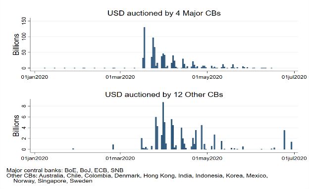
hold a large volume of US Treasuries. The pricing of this line is also more expensive than that of
bilateral arrangements.
 US dollar liquidity was actively provided to local markets through US dollar auctions by
many central banks: first in mid- to late-March, 2020 by the four major central banks, ECB, BOJ,
SNB, and BOE, then by 12 other central banks (Figure 2). The US dollar auctions by the major
central banks used US dollars obtained via swap lines with the Fed and were larger in magnitude
than the US dollar auctions by other central banks. The auctions by the other 12 central banks
that published data on these auctions, used either US dollars obtained via swap lines with the Fed
or their own foreign exchange reserves. In the case of Hong Kong, the US dollars were obtained
via the FIMA facility. 3 The US dollar shortage was mitigated by late June, so was the demand
for US dollar liquidity from major central banks (Figure 3).
 Research on the extension of swap lines during the GFC suggests that US bank exposure to
the swap partner economies and the extent of reliance on the US as their export destination are
important motivations for the Fed to extend these lines (Aizenman and Pasricha, 2010;
Aizenman, Jinjarak, and Park, 2011).
 Given that the economic environment in the COVID turmoil was different from that of the
GFC, which was a shock that originated in the US financial system, and that FIMA facility was
added as another liquidity provision scheme, one may ask whether the factors motivating the US
decision to provide dollar liquidity were different in this crisis. Did the Fed extend swap lines or
FIMA facility solely based on its self-interest as it did during the GFC? What factors determined
economies’ access to dollar liquidity? One may also ask to what extent the size of US dollar
auctions conducted by central banks reflected stress in domestic financial or currency markets.
 Other questions are also worth investigating. Are the swap lines effective in mitigating
financial stress? The announcements of swap lines during the GFC had relatively large short-run
impacts on the exchange rates of the selected emerging market economics (EMs), but much
smaller effect on the credit default swap (CDS) spreads, relative to that of other EMs that were
not the recipients of swap-lines (Aizenman Pasricha, 2010). Baba and Packer (2009) found that

3 The Hong Kong Monetary Authority announced on April 22, 2020, the launch of a US dollar
liquidity facility based on US dollars obtained via FIMA. In addition, central banks of Colombia
and Chile announced on April 20, 2020 and June 24, 2020 respectively, that they had gained
access to FIMA.

 3

US dollar term funding auctions by the ECB, SNB, and BoE, as well as the Fed’s commitment to
provide unlimited dollar swap lines ameliorated the FX swap market dislocations during the
GFC. Rose and Spiegel (2012) found that US dollar auctions by major central banks
disproportionately benefitted economies that had higher trade or asset exposure to the US, by
reducing their CDS spreads.
 We revisit these questions and investigate whether the announcement of the dollar liquidity
lines by the Fed as well as that of dollar auctions by central banks affect the performance of their
exchange rates, cross-currency basis (CIP deviations), CDS spreads, and government bond
yields. We distinguish between dollar auctions by an economy’s own central bank and those by
the five major central banks, and ask whether the impacts were different, and whether the
auctions by the major central banks had spillovers on the financial conditions in other
economies. We use a local projection model and daily data from 1 January 2020 to 31 May 2020,
on a sample of 43 economies to investigate these questions about the impact of liquidity
facilities.
 Our results indicate that an economy’s share in US trade and a military alliance with the
US are the positive factors that determined access to a Fed swap agreement. On the determinants
of the size of access to liquidity arrangements, we find that an economy with high levels of US
bank exposure and stronger trade ties with the US tended to have greater access to Fed liquidity,
via swap lines or FIMA. Economies with a large share of global trade, regardless of whether they
are major trading partners of the US, also had greater access to US dollar liquidity via the Fed.
 The access to US dollar liquidity lines was largely determined by pre-existing
characteristics of the economies. However, the demand for US dollars auctioned by central banks
should reflect the ongoing stressed in the domestic currency and financial markets. We find that
economies that faced appreciation pressures against the US dollar and whose local currency
exchange rate becomes more volatile were more likely to auction greater amounts of US dollars
in its domestic market. These effects were stronger for countries to which US had greater trade
and financial exposure. While this may sound paradoxical, the record of the GFC is that from
gold to the US dollar to the Japanese yen, ‘safe havens’ were greatly sought – and greatly
affected – by investors reacting to the global financial crisis. Thereby, the appreciation and the
volatility of the yen happened at the same time as the collapsing export/GDP of Japan during that
time.

 4

As for the effects of the announcements of swap lines and of dollar auctions by central
banks, we find that the announcement of expansionary changes in the swap arrangements and the
creation of the FIMA facility led to appreciation of non-US dollar currencies against the US
dollar, as expected. While the swap or FIMA announcements had no impact on cross-currency
basis and the 10-year government bond yields, they improved (i.e., reduced) CDS spreads.
Dollar auctions by central banks led to temporary appreciation of their currencies, but dollar
auctions by major central banks (BoE, ECB, BoJ and SNB) had persistent spillover effects – they
led to appreciation of other, non-major currencies against the US dollar. These results do not
differ for countries to which US had greater financial or trade exposure.
 Putting our results in the proper context, the conceptual differences between international
reserves and emergency swap lines and emergency liquidity arrangements are noteworthy. The
demand for international reserves is shaped by precautionary motives, i.e., ex ante insurance
against future sudden stops and trade funding challenges; and possibly concerns about trade
competitiveness, dubbed sometimes as mercantilist motives (Aizenman, 2008). In contrast,
emergency liquidity arrangements and swap lines provided during the GFC and the COVID-19
crisis provide liquidity relief at the time of crisis. Hence, there is no presumption that the
demand for international reserves are explained by the same factors determining emergency
liquidity and swap lines. At times of financial crisis, trade credits supplied by local banks may
shrink even in economies experiencing currency appreciation, as banks may opt to reduce their
risk exposure, documented by Amiti and Weinstein (2011). 4 During a deep crisis with uncertain

4 The appreciation the yen in 2008 coincided with collapsing trade credit in Japan, magnifying
the contraction of international trade at times that ‘flight to safety’ induced yen appreciation.
Amiti and Weinstein (2011) identify the presence of a causal link from shocks in the financial
sector to exporters that result in exports declining much faster than output during banking crises.
They concluded that the health of financial institutions is an important determinant of firm-level
exports during crises. Since the evidence indicates that exporters in many countries are highly
dependent on trade finance, these results imply that financial shocks are likely to play important
roles in export declines in other countries as well. Thereby, financial and trade shocks are
intertwined in different ways across countries during crises. This pattern is in line with IMF-
BAFT Survey (2009), reported by Amiti and Weinstein (2009), of 88 banks in 44 countries
revealed that the average spreads on the letters of credit, export credit insurance, and short- to
medium-term trade-related lending rose by 70, 107, and 99 basis points, respectively, in the
second quarter of 2009 relative to the fourth quarter of 2007. See also Auboin (2009) review on
trade credits before and during the GFC, noting that ‘While a number of public-institutions
mobilized financial resources for trade finance in the fall of 2008, this has not been enough to

 5

duration, like the GFC, economies may use their international reserves as a first line of defense,
but may refrain from tapping too deeply to reserves out of the fear that depleting reserves may
cost them dearly if the crisis would deepen in the future (Aizenman and Sun, 2012). In these
circumstances, swap lines and FIMA type of arrangements may mitigate the decline of trade
credit, the depletion rate of international reserves, and mitigate the rise of sovereign spreads of
exposed emerging markets.5
 Boissay, Patel and Shin (2020) indicate that the forces of these factors have only increased
after the GFC due to the dominant role of dollar funding, and the growing depth of the global
supply chains. Specifically, they noted:
 “Trade finance, as proxied by the share of cross-border factoring in total factoring, has
 steadily increased over the past two decades. This long-term trend has gone hand in hand
 with the rise in international trade and, more specifically, the lengthening of global value
 chains (GVCs). While the lengths of domestic production chains estimated using world
 input-output tables at the country-sector level have remained constant, GVCs involving
 multiple border crossings have lengthened significantly between 2000 and 2017. Since
 financing needs increase with the length of supply chains (Bruno et al (2018), Bruno and
 Shin (2019)), trade finance has become more prominent in the context of GVCs.” (page 5).
 “The sharp appreciation of the dollar in the early stages of the Covid-19 crisis may have
 had knock-on effects to trade finance from stress in the banking system. Given the
 prevalence of the US dollar in trade financing, mitigating the impact of dollar credit
 fluctuations will be an important component of shielding global value chains from the
 pandemic’s economic fallout. In this respect, the recent expansion of central bank dollar
 swap lines and other measures to mitigate dollar liquidity conditions are likely to further
 cushion trade finance.” (page 6).

 Baldwin and Freeman (2020) also highlight the magnification of the intermingling of trade
and finance associated with the of the GVC deepening. The COVID pandemic vividly illustrated
the dependence of the US and the EU on the GVC as the source of critical medical supplies.
These considerations imply that we should take the econometric significance of the ‘trade

bridge the gap between supply and demand of trade finance worldwide. As the market situation
continued to deteriorate in the first quarter of 2009, G-20 leaders in London (April 2009) adopted
a wider package for injecting additional liquidity and bringing public guarantees in support of
$250 billion of trade transactions in 2009 and 2010.’
5 If the economy of concern is long in dollar assets (e.g., Japan, Germany, Switzerland), its

currency’s appreciation would induce valuation losses in terms of its domestic currency (in
addition to adverse impacts on international trade), magnifying the losses on the US equities and
putting more pressure on the economy’s balance sheet. Hence, even with its currency
appreciation, financial instability may arise.

 6

factors’ in our regressions with a grain of salt: one needs micro data to identify more sharply the
role of trade, finance and the interaction between the two.
 The results of our paper also are in line with Gourinchas and Rey (2007), Obstfeld et al.
(2009), and Gopinath et al. (2020), analyzing the “exorbitant privilege” position of the US dollar,
and the dominant currency paradigm. These considerations suggest that the FEDs swap lines
and emergency liquidity provisions of the FIMA type may impact most emerging and developing
economies, including nations with limited trade and financial dealings with the US. For
economies with greater trade and financial integration with the US, these effects tend to be more
direct, for others, in the form of spillovers.
 The paper is organized as follows. In Section 2, we first reexamine what factors led the Fed
to select nine countries as swap partner countries as it did during the GFC. We then investigate
the determinants of the size of liquidity lines – both swap and FIMA- in Section 3. In Section 4,
we examine the determinants of the size of dollar auctions by central banks. In Section 5, we
examine the impact of the liquidity lines and dollar auctions by central banks on important
financial variables. In Section 6, we present the results of numerous robustness checks. In
Section 7, we make concluding remarks.

2. Probability of gaining access to Fed swap lines

 The COVID-19 crisis saw a re-emergence of dollar liquidity shortages around the world, as
evidenced by the widening of the cross-currency basis between the US dollar and other
currencies (Figure 1). While the Fed reactivated swap lines with the same nine central banks with
which it had established them in 2008. However, considering the difference in the economic
conditions between the GFC and the COVID crisis as well as the difference in terms of the type
of shock that hit the world economy (i.e., financial crisis originating in the US vs. the pandemic),
the determinants for the selection of the nine central banks may differ between the two crisis
episodes.
 Hence, it is worthwhile to examine what factors led the nine central banks to be selected to
receive swap liquidity lines from the Fed again. Following Aizenman and Pasricha (2010), we
estimate the factors that affect the probability of economies included in the swap agreements.
The candidate factors are: exposure of US banks to individual economies (BankExp), measured

 7

by the share of the individual market in the consolidated foreign claims of US banks; trade
exposure to the US (TradeShare), measured by the share of economy i in total US goods imports
and exports; financial openness (KAOPEN) measured by the Chinn-Ito index of capital account
openness (2006, 2008); and the existence of formal military relationship with the US
(ALLIANCE).
 By extending US dollar liquidity to economies where US banks have greater asset
exposure, the Fed could prevent costly deleveraging, possibly enhancing the welfare of both -
source and recipient - economies. The more trade economy i conducts with the US, the greater
the incentive of the Fed to secure trade flow by readily granting liquidity lines to the economy. A
more financially open economy might have more need of liquidity lines, as the size of financial
shock it faces may be larger due to its greater integration with global financial system. A non-
economic factor may matter: the US may prefer providing swap lines with economies it has
closer geopolitical relationship.
 We apply the probit estimation model to a sample of 77 economies, based on data
availability. This sample does not include Canada, the euro countries, Japan, Switzerland, and
the United Kingdom because these countries have standing swap lines with the Fed. The
dependent variable is a dummy variable that takes the value of unity when the economy of
concern is selected as the recipient of swap lines. All the explanatory variables are sampled as of
the end of 2019.
 Columns of (1) through (4) of Table 2 show that all the candidate variables are significant
contributors to selection into Fed’s swap agreements when they are included alone. Greater US
banks’ exposure, greater US trade exposure, more open financial markets, and the existence of
military alliance increase the probability of receiving a Fed swap line. Among the three
variables, the dummy for a military relationship with the US alone explains the probability of
providing a swap line the most (pseudo R2 of 18%).
 Columns (5) through (7) include the dummy for military alliance and two of the remaining
three variables. Among the three models, the model in column (6), with US trade exposure and
de-jure financial openness of the economy, yields the highest pseudo R2, though the estimate on
financial openness becomes statistically insignificant. When we include all the candidate
variables in the estimation, the variables for the share in US trade and military alliance maintain
statistical significance. Financial exposure may contribute positively to the probability of

 8

selection for the swap arrangement, but its contribution is not as significant as that of US trade
exposure.
 u rfin d in g s a p p e a rto b e d ife er n t fro m ize n m a n a n d a srich a () w ith re sp e ct to th e im p o rta n t o f tra d e e x p o su er .ize n m a n a n d a srich a () fo u n d th a t b a n k e x p o su re w a sa sig n ifca n tly p o sitv e co n trib u to r to th e se le ctio n o f e m e rg in g m a rk e tsfo r sw a p a g re e m e n ,b
 ts u t tra d e e x p o su re w a s n o t.n e re a so n fo r th is d ife re n ce m a y b e th a th e fin a n cia l cris o rig in a te d in th e a n d th re a te n e d th e so lv e n cy o fb a n k in g in stiu tio n .s h e re fo re th
 , e sw a p lin e s th e n w e re a im e d a t p ro v id in g liq u id ity lin e s to th e e co n o m ie w
 s h e re b a n k e x p o su re w a sh ig h . u rin g th e - cris, d e sp ite la rg e -sca le fa ls in th e sto ck m a rk e ts a n d w id e sp re a d d o la rsh o rta g e , th e re w a s n o a cu te sy est m a ict fin a n cia l in sta b ilty a d
 s u rin g th e .o w e v e r,d u rin g th e - cris, g lo b a lsu p p ly ch a in s g o set v e re ly d isru p te d . e v e ra lp a p e rsh a v e h ig h lig h te d th e in cre a sin g im p o rta n ce o f g lo b a lv a lu e ch a in sin th e p a st tw o d e ca d e sa n d th e a so cia te d in te rm in g lin g o f tra d e a n d fin a n ce (o isa y , a te la n d h in , ; a ld w in a n d re e m a n ).; h e p a n d e m ic

v iv id ly ilu stra te d th e d e p e n d e n ce o th
 f e a n d th e o n th e a s th e so u rce o f crita l m e d ica l su p p lie s, a n d th e sh a rp a p p re cia tio n o fth e d o la r in th e e a rly sta g e s o fth e o v id -cris m a y h a v e h a d k n o ck -o n e fe ctso tra d e fin a n ce fro m stre s in th e b a n k in g sy ste m . h e se co n sid e ra tio n s im p ly th a t w e sh o u ld ta k e th e e co n o m e tric sig n ifca n ce o f th e ‘trad e fa cto rs’ in o u re g re o
 si n s w ith a g ra in o fsa lt: o n e n e e d sm icro d a ta to id e n tify m o re sh a rp ly th e ro le o f tra d e ,fin a n ce a n d th e in te ra ctio n b e tw e e n th e tw o .

3. Determinants of the size of liquidity lines via swap agreements and FIMA

 While the number of economies that have swap agreements with the US is limited (i.e., 14
in total with five central banks with long-standing arrangements and nine reactivated), the newly
created FIMA facility is available to economies which do not have any swap agreements as long
as they hold stocks of US Treasuries in their foreign exchange reserves which they can swap for
dollars in the repo transactions. Therefore, the sum of the maximal amount of swap agreement
with the Fed and the amount of US Treasuries in the foreign exchange reserves holding of an
economy can be regarded as the potential availability of liquidity lines from the Fed. We
estimate the determinants of the total size of liquidity lines available.
 The size of liquidity lines available to economy i, , is composed of swap lines, ,
and the FIMA line, , namely,

 = + . (1)

 We investigate the determinants of the available amount of liquidity lines using the
estimation model below:

 ′
 = + + (2)

where is the available amount of dollar liquidity and X’i is a vector of candidate explanatory
variables.
 As for the size of the swap lines, SWAPi is straightforward because it is stipulated in the
agreements. The maximal amount of swap lines is $60 billion each for the RBA, BCB, BOK,
BdM, MAS, SR, and $30 billion each for the DNB, the NB, and RBNZ. We do not include the
economies of the following five central banks: the BOC, BOE, BOJ, ECB, and SNB, in the
estimation because there is no limit to the swap lines for these central banks.

 9

Measuring the size of liquidity lines through the FIMA facility is not straightforward
because there is no stipulation about the available amount of liquidity lines through the facility.
Instead, the FIMA repo facility allows foreign central banks and other international monetary
authorities to temporarily exchange US Treasuries held in their accounts at the Federal Reserve
Bank of New York for US dollars. Hence, the amount of dollar-denominated reserve assets is a
good proxy for the dollar liquidity available to economy i.
 To measure US dollar-denominated reserve assets, we need the data on the volume of
reserve assets held by central banks and their currency composition. However, such data is
notoriously limited. 7 Recently, Ito and McCauley (2020) compiled a panel dataset on the shares
of key currencies in foreign exchange reserves for about 60 economies in the 1999-2018 period. 8
In order to obtain the holdings of dollar-denominated reserve assets, as an approximate of the
availability of liquidity lines through FIMA, we multiply the dollar share in foreign exchange
reserves as of 2018 from the Ito-McCauley dataset, with total reserves (minus gold) as of 2019. 9
 The candidate factors that may affect the availability of liquidity lines include the variables
we tested in the previous exercise, namely, US bank exposure, the share of trade with the US,
military alliance, and de jure financial openness. From the perspective of the US, it is rational to
build a system that can provide liquidity lines for the economies that have more loans from US
banks or that have more trade with the US.
 In addition to these variables, we also test the variables for global financial exposure and
the share of the economy in world trade. The rationale to test these variables is that the US might
be willing to provide liquidity lines for the economies that do not necessarily have stronger
financial or trade ties with the US per se. In other words, the US could be “altruistic” and willing
to play the role of the guardian of the international economy by making dollar liquidity readily
available through swaps or FIMA facility for large players in international finance or trade. We
measure the level of global financial exposure (Global_Fin i) with economy i’s sum of external

7 Heller and Knight (1978), Dooley et al (1989), and Eichengreen and Mathieson (2000) use the
International Monetary Fund’s (IMF) currency composition of official foreign exchange reserves
(COFER). However, the data for individual countries are not publicly available.
8 Ito and McCauley (2020) collected the data from central banks’ annual reports, financial

statements, and other publicly available information sources.
9 If the 2018 data is not available, the dollar share data as of 2017 is used. The data availability

for this exercise is determined by the Ito and McCauley dataset. Therefore, this regression
exercise covers 51 economies.

 10

assets and liabilities as a ratio to the world’s external assets and liabilities over the period of
2005 through 2015, using the database compiled by Lane and Milesi-Ferretti (2001, 2007, and
2017). While a significantly positive estimate on BankExp would imply that the US is more self-
interested to make dollar liquidity readily available for economies with more consolidated claims
of US banks, a significantly positive estimate on Global_Fin i would mean that the US is willing
to make dollar liquidity available for economies playing a larger role in global finance. Parallel
to Global_Fin i, the variable of global trade exposure (Global_Tradei), measured by the share of
economy i’s sum of exports and imports in global trade (i.e., the world’s sum of exports and
imports), would show whether or not the US is altruistic to maintain global trade order by
providing liquidity to economies that have larger presence in international trade.
 We also test the dummy for China since the country’s holding of dollar-denominated assets
is by far larger than the rest of the sample economies. As in the previous exercise, all the
explanatory variables are sampled as of the end of 2019. We run a cross-sectional OLS
regression for 51 economies.
 The results presented in Table 3 indicate that higher US bank exposure to an economy led
to a greater liquidity from the swap agreement. Interestingly, the variable for US bank exposure
alone explains 20% of the variation of the availability of dollar liquidity. Also, an economy with
more trade with the US tends to have more accessibility to dollar liquidity, additionally
explaining another 77% of the variation of dollar liquidity availability. Just the two variables of
US bank exposure and the share in US trade explain 97% of the variation of the accessibility of
dollar liquidity, perhaps because they determine the amount of dollar-denominated assets held in
FX reserves.
 Columns (3) through (6) also indicate that the US is altruistic in the sense that it makes
dollar liquidity available for global major trading centers regardless of whether those economies
are major trading economies with the US However, the share in global finance does not matter
for liquidity accessibility. These findings suggest that, as we found in the previous exercise, trade
plays an important role in terms of determining which economies have better access to dollar
liquidity. The estimates of the three variables, US bank exposure, the share in trade with the US,
and global presence of trade, are persistently statistically significant across the different models
and explain almost all of the variation in the availability of dollar liquidity. The extent of
financial openness does not matter for the size of dollar-liquidity available. China appears as an

 11

outlier, but inclusion of the dummy does not materially change the estimates of the other
variables (not reported).

4. Determinants of the size of US dollar auctions by central banks

 The actual use of liquidity lines may differ from the availability of liquidity lines. Both the
availability and the use of US dollar liquidity may affect market perceptions and conditions,
which we will investigate in section 4. In this section, we investigate the factors that determine
the amount of US dollars auctioned by central banks in their domestic markets. Most of these
auctions used the Fed liquidity lines as the source of the US dollar auctioned by central banks.
The amount of dollars auctioned was largely determined by market conditions.10
 We regress the amount of US dollars auctioned on a set of candidate variables. They
include: cumulative depreciation (Cuml_fx), which is the rate of change in the local currency
value per dollar with respect to the average local currency value during the first two weeks of
January 2020; exchange rate volatility (fx_vol), the standard deviations of the rate of depreciation
over rolling 14-day windows; stock market volatility (stk_vol), the standard deviations of the rate
of stock market total return over rolling 14-day windows; the level of financial instability
measured by the Chicago Board Options Exchange Volatility Index (VIX) in log; and US Bank
exposure (BankExp) to these economies as of 2019Q4. We also test the variable for the number
of new cases of COVID infection (COVID) measured by the moving average coronavirus
infection cases per million over 7 days, and the mobility index (MOBILITY) to capture the
possible impact of economic activities on daily basis. The estimation model also includes
interactions of US bank exposure with cumulative depreciation and exchange rate volatility. For

10Some central banks, including the major central banks, either did not notify a maximum limit
on the auctions, or notified an amount large enough that the amount auctioned was determined
by the bids received. There were only a few cases – in Colombia, India, Indonesia, and Mexico –
where the amount bid was larger than the amounts notified, and therefore accepted, by the
central banks.

 12

this estimation, we apply an OLS estimation model to the daily panel data of 42 economies for
the period of January 15, 2020 through May 29, 2020. 11,12

 The estimate on the cumulative depreciation rate is significantly negative, in the results
reported in columns (1) and (2) of Table 4. This suggests that central bankers facing their
currency appreciating cumulatively compared to the beginning of January 2020 auctioned more
US dollars in their domestic markets. The estimate on the variable for exchange rate volatility is
significantly positive, suggesting when their currency’s value is unstable, central bankers auction
more US dollars. More global financial instability also increased the amount of US dollars
auctioned by the monetary authorities. In column (2), we add the interaction term between the
cumulative depreciation rate and US bank exposure as well as the interaction term between
exchange rate volatility and US bank exposure. The results indicate that the reaction to
cumulative depreciation or exchange rate volatility is greater for economies to which US banks
has greater exposure.
 In model 3, we include the variable for the number of new COVID cases and the mobility
index both of which are more directly related to the pandemic. Only the variable for new COVID
cases is found to be a significant factor.

5. The economic impacts of Federal Reserve liquidity lines and US dollar auctions
 While providing dollar liquidity through a swap agreement or the FIMA facility can have
economic impacts through alleviating dollar liquidity shortage, the mere announcement of these
liquidity facilities can also have economic impacts because such a policy announcement would
affect economic agents’ expectations and consequently their behavior (confidence channel).

11 One may suggest that we should use the Heckman two-step selection model (1976), in which
the first step is the probit estimation of the probability of auctioning and the second step is the
OLS to estimate the amount of the auctions. However, as Table 1 makes it clear, the timing of
auctions is pre-announced, i.e., it is not determined by economic and non-economic conditions. It
is rather determined mechanically. Hence, we think estimating the probit model prior to the OLS
estimation is inappropriate.
12
 This regression includes the Euro-area. We compute GDP-weighted Euro-area averages of
stock price volatility, new COVID-19 cases per million and mobility indices. For US bank
exposure, we use the unweighted sum over all Euro-area countries.

 13

In this section, we investigate whether and how the announcements of the swap
agreements or the creation of the FIMA facility affect economic variables, namely, credit default
swap (CDS) spread, the absolute cross currency basis (absolute deviations from covered interest
parity) relative to its average 2019 level, government bond yields, and the local currency
exchange rate while controlling for other domestic and international economic conditions and
policies. We also examine the domestic and spillover effects of US dollar auctions held by
central banks, and whether these effects are greater for economies that are more exposed to the
US in terms of trade or financial transactions.

5.1 Baseline model
 To capture the size and the persistence of the impacts on economic variables, we employ
the local projection method (Jordà, 2005) to the sample of 43 economies and run a series of
regressions for different horizons, r = 0,1,2,…, p as follows (IMF, 2020): 14, 15

 , , 
 ∆ , −1→ + = � 1 , + − + � 2 , + − 
 =0 =0

 , , 
 + ∑ =0 3 + ∑ =0 4 , + − 
 , + − 

 3 3 3

 + � 1 , − + � 2 , − + � 3 
 , − 
 =1 =1 =1

 + ∑3 =1 4 , − + − + + + , + 

 (3)

14 The sample includes Canada, the U.K., Japan, Switzerland, and the euro area. We compute
GDP-weighted euro area averages of government bond yields, CDS spreads, new COVID-19
cases per million and mobility indices. For US bank exposure, we use the unweighted sum over
all euro area countries. For sovereign rating changes, the variable takes the value 1 if there is an
upgrade to any euro area country on that day, and -1 for any downgrade.
15 The model framework also follow Teulings and Zubanov (2014) who include not just the
 , 
lagged variables of control variables but also their leads (i.e., ∑ =0 , + − where X is an
explanatory variable). They argue that it would prevent the estimates from being biased.

 14

∆ , −1→ + is the cumulative percentage point change from t-1 to t+p in economy i’s currency
per US dollar; absolute cross-currency basis differential for economy i’s currency against US
dollar; economy i’s 10-year sovereign bond yield; or the credit default swap (CDS) spread for
economy i.
 Swapfima is a dummy variable that takes the value of one on the days of Fed swap
announcements for swap recipients, and on the day of the FIMA facility announcement for all
economies. That is, when the Fed makes an expansionary change in the swap policy, the dummy
takes the value of one for the counterpart economy in the swap agreement. For example, the Fed
reduced swap pricing and introduced 84-day operations with five major central banks on March
15, 2020. On March 19, the Fed reactivated swap lines with nine central banks. On March 20,
BoC, BoE, BoJ, ECB, and SNB took a coordinated action to enhance the effectiveness of the
standing dollar swap by increasing the frequency of 7-day maturity operations from weekly to
daily. Swapfima takes the value of one for relevant counterpart economies and swap
announcement dates. When the FIMA facility was created on March 31, 2020, in contrast, the
dummy variable takes the value of one for all the sample economies because this policy is
relevant all economies. All these policy actions are meant to provide more dollar liquidity and
therefore stimulative actions.16
 In the baseline specifications, Auction Own is the dummy for the dates when economy i’s
central bank auctions of US dollars whereas AuctionMajor is a dummy that takes the value of one
for the dates when major central banks (ECB, BOE, SNB, and BOJ) auctioned US dollars. This
variable aims to capture the spillover effects of auctions by the major central banks. In
robustness checks, we redefine, Auction Own and Auction Major to use the auction amounts (the
amounted accepted in the auctions) instead of dummies for auction days.
 The model controls for other stimulus policies that are supposed to affect liquidity and
include the following variables in the vector Other Controls: QE is the dummy for quantitative
easing (QE) implemented by the Fed on March 23. NPR is a decline in the monetary policy rates
of the sample economies (i.e. the negative of the change in the policy rate). We also control for

16 We decided not to assign a separate dummy for each of the Fed policy actions. Because these
policies were implemented on close dates to one another, the impact of individual policy actions
is difficult to identify – the lags and leads in the estimation model make it more difficult.

 15

global financial market conditions using the Chicago Board Options Exchange Volatility Index
(VIX) in log. We control for changes in sovereign credit ratings by any of the big three credit
rating agencies, Standard and Poor’s, Moody’s, or Fitch. The variable for the change in
sovereign credit ratings takes the value +1 on the days when there is a ratings upgrade by any of
the agencies, -1 for the days with a downgrade, and 0 otherwise. As another factor that can affect
expectations, we control for the pandemic situation with the first lag of the 7-day moving
average of new corona cases per million (COVID).
 The estimation includes economy fixed effects and weekly time fixed effects is conducted
for business days for the period of January 2 through May 31, 2020.17 We employ the local
projection method that estimates a series of regressions for each horizon p for each variable.
Here, we assign p to be 5, that means we attempt to capture the full dynamics of each of the four
dependent variables in the aftermath of policy announcements or actions by central banks over
the course of five business days. Standard errors are robust. To focus on the dynamics of the
economic variables in response to a policy shock, we focus on reporting the cumulative impulse
response functions (IRFs) rather than discussing the estimated coefficients.18
 We have two practical reasons to use the local projection model over the VAR model. First,
to economize the number of estimates, we employ two-way fixed effects, namely, economy-
fixed effects and weekly time fixed effects. Including these fixed effects in a VAR model would
complicate the estimation. Economy-fixed effects control for time-invariant, or slowing
changing, characteristics of each sample economy (e.g., the level of development of the medical
and insurance systems, economies’ debt levels, the tendency for fiscal interventions). Weekly
fixed effects control for common, global waves of the virus infections or related news. Including
these fixed effects helps reduce the number of estimated parameters. These fixed effects also
allow us focus on the estimates of the variables of our interest, i.e., the dummies for the
announcements or the implementation of swap and other stimulus policies. These fixed effects

17The first policy action related to swap operations took place on Sunday, March 15. To capture
the impact of the policies, we assign the value of one in Swapfima on March 16.
18Auerbach and Gorodnichencko (2013), Ramey and Zubairy (2018), Sever and others (2020)
and many others have applied the local projection model to macroeconomic analyses.

 16

are easier to include in the estimation model and to interpret when the local projection model is
used, but not so much with a VAR model.
 Second, using the IRF based on the local projection model is more appropriate when the
estimation involves nonlinear estimates. As we discuss later, we test whether the impact of swap
and other stimulus policies varies with US trade or financial exposure with the recipient
economies. To test this, we include interaction terms between US trade or financial exposure and
the policy variable of our interest. While nonlinear VAR models exist, the estimation and
interpretation of their estimates is highly complex. With the local projection model, this kind of
exercise can be done with ease.

5.2 Baseline results: Announcement effects of Federal Reserve liquidity lines

 The main purpose of Fed swap lines or the FIMA facility was to increase US dollar
liquidity globally and stabilize foreign dollar markets. Panel (a) of Figure 4 shows that the
currencies of recipient economies appreciate on the day of the policy announcement and days 4
and 5, which means that the US dollar depreciates against these currencies on those days,
consistent with the policy objective. The announcements of swap lines or FIMA do not seem to
affect the absolute three-month cross-currency basis differential, which is a more direct measure
of market dislocations (Figure 4(b)). However, it must be noted that the data for this variable is
available for only 21 currencies. The finding that the US dollar depreciates against the currencies
of swap/FIMA recipients following the announcements of these policies does signify that the
policies mitigated the dollar shortage.
 The CDS spreads for swap/FIMA recipients improve when the Fed shows its willingness
to provide dollar liquidity (Figure 4(c)). The persistent decline in the CDS spreads starts
immediately on the day when the policy is announced, and the spread improvement lasts for the
following two business days. We can interpret this finding as evidence that the (expected)
mitigation of dollar constraint would reduce the default risk in general.
 Fed swap lines could have an expansionary impact on the long-term interest rates of
recipient economies, through a reduction in default risk. Figure 4(d) shows that the
announcements of swap lines put downward pressure on the ten-year government bond yields,
but the impact is not statistically significant.

 17

The estimated impacts of other variables are also consistent with theoretical predictions.
For example, a rise in VIX leads to a relatively large depreciation of the home currency, of about
2 percentage points, which lasts 3 days (Figure 5(a)). This reflects a tendency for investors to
rush into dollar-denominated assets when the financial markets are exposed to a negative global
shock, which leads to dollar appreciation. Quantitative easing (QE) by the Fed, on the other
hand, leads to a persistent and large appreciation of the other currencies and a US dollar
depreciation, as expected. The expected result can also be observed in the estimated impact of
QE on the non-US ten-year government bond yields (Figure 5(b)). Neither VIX nor QE seems to
have any impact on the CDS spread (Figure 5(c)). A fall in the domestic monetary policy rate
does not have a significant impact on any of the economic variables, consistent with the results
in Sever and others (2020).

5.3 Domestic and spillover effects of US dollar auctions

 This estimation model also allows us to examine the impact of central banks’ swap
auctions to supply dollar liquidity to the markets, on financial variables. Most of the auctions are
pre-announced, and often, but not always, the source of dollars being auctioned is from the
Federal Reserve swap lines or FIMA. 19 We assess the impact of US dollar auctions by economy
i’s own central bank/monetary authority on the economic variables of our interest. We also
examine the spillovers of US dollar auctions by the four major central banks (i.e., BOE, BOJ,
ECB, or SNB) on other economies’ financial variables.
 On the days when the central banks of our sample economies conduct US dollar auctions,
their home currencies appreciate on days three and four, perhaps reflecting the first settlement of
the auctions, but the cumulative effect is not significant on day 5. (Figure 6 (a)). Own central
banks’ dollar auctions therefore have a short-lived effect of alleviating pressure on the domestic
currency. When any of the major central banks conducts FX auctions, on the other hand, there is
an immediate appreciation of other economies’ currencies against the US dollar, with its impact
persistently becoming larger through day 5. These findings suggest that foreign exchange swap

19For example, the Reserve Bank of India announced that it will conduct US dollar auctions on
March 12, 2020, without specifying the source of the US dollars, which likely were from its own
reserves, as FIMA had not yet been announced and the RBI does not have swap line with the
Fed. The Hong Kong Monetary Authority announced on April 22, 2020 that it will conduct US
dollar auctions using funds obtained from the FIMA.

 18

auctions by the major central banks are very effective and have implications beyond the home
economies.
 FX auctions do not appear to affect the dynamics of the ten-year government bonds yields
or the CDS spread, except for a small but short-lived ameliorative impact of major central bank
auctions on government bond yields of other economies (Figures 6 (b), (c)).

5.4 Interactive analysis: Does US-exposure matter for impact of dollar auctions?

 How the US dollar swap or auction policies affect the dynamics of the economic variables
of our interest can depend on whether and to what extent the economies are exposed to the US in
terms of trade or financial transactions. Rose and Spiegel (2012) find that the impact of swap
auctions of dollar assets by foreign central banks is larger for economies that have more trade or
financial linkages with the US.
 We now examine whether and to what extent the level of trade or financial linkage with the
US affects the impact of US dollar swap or auction policies by including in the estimation model
the interaction terms as:

 , , 
 ∆ , −1→ + = � � , + − + � � , + − ∙ 
 =0 =0

 3 
 
 + � � , − + � � , − ∙ + − + + 
 =0 =0

 + , + (4)

where EXP is either BankExp (exposure of US banks to individual economies) or TradeShare
(the share of economy i in total US goods imports and exports).20 The estimates of our focus are
 , 
 . If the extent of trade or financial exposure matters, this estimate will be significant with a
sign that would enlarge the absolute magnitude of Swampfima or other policy shock variables

20We do not include the level term of EXP, mainly because the preliminary test showed that
neither BankExp nor TradeShare enters the estimation significantly. Rose and Spiegel (2012) do
not include the level terms for the same reason.

 19

(i.e., FIMA announcement, and own or major central bank auctions). are each of the
explanatory variables in the baseline model other than COVID, i.e. Swapfima, Auction Own,
Auction Major and Other Controls.
 Figure 7 (a) illustrates the interactive effects of swap-related policies and bank exposure.
 , , 
That is, � 1 + 1 ∙ , + − � ∙ , + − when EXP is BankExp. To make the
interpretation easier, we draw two lines, one for the case where BankExp takes the 75 th percentile
value (blue line) and the other for the 25th percentile value (red line). From the two lines barely
apart from each other, we can see that the extent of bank exposure does not affect the impact of
 , 
Swampfima. ̂1 is statistically insignificant. The impacts of swap auctions by either individual
economies’ central banks or the major central banks do not depend upon bank exposure. The
lack of statistical significance is not just the case for the impacts on the exchange rate, but also
 , 
on the sovereign debt yield or the CDS spread (Figures 8 and 9). In fact, most of ̂ turn out to
be statistically insignificant. 21
 , 
 When we include TradeShare for EXP, again, in most of the cases, ̂ is statistically
insignificant, indicating that the extent of trade exposure to the US does not affect the impact of
swap policies or auctions.
 These estimation results give us an answer to the question of whether the effects of
liquidity-providing policies differ depending on the extent of trade or financial exposure to the
US The answer is no. This finding is different from that of Rose and Spiegel (2012). We
conclude that US liquidity-providing policies are indiscriminatory, possibly benefiting
economies regardless of the existence of trade or financial ties with the US That is consistent
with the claim that the US Fed is the lender of the last resort.

6. Robustness checks

 The results presented in section 5 are robust to several changes in specification. 22 First, we
increased the number of lags and leads in the model to 11 leads and 6 lags. The results remain
robust, and the announcement effect of the swap lines and FIMA on exchange rates against the

21 Therefore, to avoid the figure cluttered with many lines, we do not show confidence intervals.
22 The results are available on request.

 20

US dollar persists on day 11, while the impact of the auctions by the major central banks persists
until day 10.
 Second, the estimation results are robust to using alternative control variables that measure
the severity of the pandemic. We used total number of COVID-19 cases instead of new cases per
million, controlled for lockdowns and for changes in the level of mobility with respect to the pre-
pandemic period. These variables are not significant, and do not affect the results for the
variables of interest as described in the previous section.
 Third, we used the US dollar amounts auctioned by central banks (i.e. the US dollar value
of bids accepted) instead of the dummy to represent the days when auctions took place. When we
use the auction amounts rather than the auction dummies, we find that the auctions by own
central banks briefly reduce the absolute cross-currency basis differential, indicating a brief
alleviation of market dysfunction, but auctions by major central banks continue to show no
significant impact. The results for the other variables remain unchanged from those descried in
section 5.

7. Concluding remarks

 The outbreak of the COVID-19 pandemic instigated a financial turmoil in March 2020. As
in the previous episodes of financial instability, the uncertainty made investors rush to hold US
dollar-denominated assets, creating a dollar shortage. To prevent this situation from morphing
into a global systematic financial crisis, the Fed made US dollar liquidity readily available
through reinforcing or reactivating central bank swap lines and creating the FIMA repo facility.
 This paper investigates the motivations for and effects of US dollar liquidity provision with
the following questions: First, what factors led the Fed to select nine economies as swap partners
as it did at the time of the GFC? Second, what factors determined the total availability of
liquidity lines (swaps and the FIMA facility) from the Fed? Third, what domestic conditions
determined the size of dollar auctions by central banks? Fourth, what were the announcement
effects of the Fed liquidity arrangements? Fifth, what were the domestic and spillover effects of
dollar auctions by central banks? Sixth, did the economic impacts of the US dollar liquidity
provision differ depending on the degree of US financial or trade exposure?

 21

We find that the Fed chose to reactivate swap agreements with nine economics because of
these economies’ large trade ties with the US. This result is in contrast with the previous episode
of dollar shortage in 2008 when the US signed swap agreements with emerging economies due
to their financial ties with the US. The existence of formal military alliances was also a
determinant for the Fed to reactivate the swaps for these economies. Economies with strong
financial and trade ties with the US tended to have more access to dollar liquidity lines. Global
major trading centers also had greater access to US dollar liquidity via the Fed, regardless of
whether they had more financial or trade ties with the US. The amounts auctioned by central
banks were larger for currencies that faced greater exchange rate volatility, and when global
financial conditions were more unstable, as captured by a higher VIX.
 The announcements of swap-related policies had meaningful impacts on economic
variables; they led to appreciation of the partner currencies against the US dollar, and a decline
in the economies’ CDS spreads and ten-year government bond yields. US dollar auctions by
economies’ own central banks led their home currencies to appreciate. Although this effect was
temporary. US dollar auctions by the major central banks (BoE, ECB, BoJ and SNB) had more
persistent appreciation effects on the home currencies of the non-major economies. That
indicates that liquidity policies taken by the major central banks have important spillover effects
on other economies.
 One may conjecture that the economic impacts of swap and other liquidity policies or
auctions can be greater for the economies to whom US had greater financial or exposure.
However, our findings suggest that dollar liquidity policies have egalitarian impacts irrespective
of the extent of financial or trade ties of the US.

 22

References

Aizenman, J., 2008. Large hoarding of international reserves and the emerging global economic
 architecture. The Manchester School, 76(5), pp.487-503.
Aizenman, J., Y. Jinjarak, and D. Park. 2011. “International Reserves and Swap Lines:
 Substitutes or Complements?” International Review of Economics and Finance, 2011,
 20:1, pp. 5-18.
Aizenman, J., and G. K. Pasricha. 2010. “Selective Swap Arrangements and the Global Financial
 Crisis,” International Review of Economics and Finance, 19(3), 353-365.
Aizenman, J. and Y. Sun. 2012. “The financial crisis and sizable international reserves depletion:
 From 'fear of floating' to the 'fear of losing international reserves'?” International Review of
 Economics and Finance, 2012, 24, pp. 250-269.
Amiti, M., & Weinstein, D. E. 2011. Exports and financial shocks. The Quarterly Journal of
 Economics, 126(4), 1841-1877.
Amiti, M. and Weinstein, D.E., 2009. Exports and Financial Shocks. NBER Working Paper,
 (w15556).
Auboin, M., 2009. Restoring trade finance during a period of financial crisis: Stocktaking of
 recent initiatives (No. ERSD-2009-16). WTO Staff Working Paper.
Auerbach, Alan J., and Yuriy Gorodnichenko. 2013. “Fiscal multipliers in recession and
 expansion.” Fiscal policy after the financial crisis. University of Chicago Press. 63-98.
Baba, N., and F. Packer. 2009 “From Turmoil to Crisis: Dislocations in the FX Swap Market
 Before and After the Failure of Lehman Brothers,” Journal of International Money and
 Finance, 28, 1350-1374.
Baldwin, R. and Freeman, R., 2020. Supply chain contagion waves: VoxEU, 01 April.
Boissay, F., Patel, N., and Shin, H.S., 2020. Trade credit, trade finance, and the Covid-19
 Crisis. BIS Bulletin No. 24, 19 June 2020.
Chinn, M. D., and H. Ito. 2006. What Matters for Financial Development? Capital Controls,
 Institutions, and Interactions. Journal of Development Economics 81(1): 163–192.
Chinn, M. D., and H Ito. 2008. A new measure of financial openness. Journal of Comparative
 Policy Analysis, vol 10, no 3), pp 309–322.
Dooley, M., S. Lizondo and D. Mathieson. 1989. “The currency composition of foreign
 exchange reserves”, IMF Staff Papers, vol 36, pp 385–434.
Du, W., A. Tepper, and A. Verdelhan. 2018. Deviations from covered interest rate parity. Journal
 of Finance 73 (3), 915–957.
Eichengreen, B. and D. Mathieson. 2000. “The currency composition of foreign exchange
 reserves: retrospect and prospect”, IMF Working Papers, no WP/00/131, July.
Frankel, J and S-J Wei. 1996. “Yen bloc or dollar bloc? Exchange rate policies in East Asian
 economies”, in T Ito and A Krueger, eds, Macroeconomic linkage: savings, exchange rates,
 and capital flows, Chicago: University of Chicago Press, pp 295–329.
Gopinath, G., Boz, E., Casas, C., Díez, F.J., Gourinchas, P.O. and Plagborg-Møller, M., 2020.
 Dominant currency paradigm. American Economic Review, 110(3), pp.677-719.

 23