Bitcoin pricing: impact of attractiveness variables - Financial Innovation
←
→
Page content transcription
If your browser does not render page correctly, please read the page content below
Hakim das Neves Financial Innovation
https://doi.org/10.1186/s40854-020-00176-3
                                           (2020) 6:21
                                                                                                                        Financial Innovation

 RESEARCH                                                                                                                                   Open Access

Bitcoin pricing: impact of attractiveness
variables
Rodrigo Hakim das Neves

Correspondence: rodrigohakim@
hotmail.com                           Abstract
Sao Paulo School Of Economics
(FGV), Sao Paulo, Brazil              The research seeks to contribute to Bitcoin pricing analysis based on the dynamics
                                      between variables of attractiveness and the value of the digital currency. Using the
                                      error correction model, the relationship between the price of the virtual currency,
                                      Bitcoin, and the number of Google searches that used the terms bitcoin, bitcoin crash
                                      and crisis between December 2012 and February 2018 is analyzed. The study also
                                      applied the same analysis to prices of Bitcoin denominated in different sovereign
                                      currencies traded during the same period. The Johansen (J Econ Dyn Control 12:231-
                                      254, 1988) test demonstrates that the price and number of searches on Google for
                                      the first two terms are cointegrated. This research indicates that there are strong
                                      short-term and long-term dynamics among attractiveness factors, suggesting that an
                                      increase in worldwide interest in Bitcoin is usually preceded by a price increase. In
                                      contrast, an increase in market mistrust over a collapse of the currency, as measured
                                      by the term bitcoin crash, is followed by a fall in price. Intense world economic crisis
                                      events appear to have a strong impact on interest in the virtual currency. This study
                                      demonstrates that during a worldwide crisis Bitcoin becomes an alternative investment,
                                      increasing its price. Based on it, bitcoin may be used as a safe haven by the financial
                                      market and its intrinsic characteristics might help the investors and governments to
                                      find new mechanisms to deal with monetary transactions.
                                      Keywords: Bitcoin pricing, Price variables, Crisis

                                    Introduction
                                    Concurrent with a rapid price appreciation, the increase in financial market interest in
                                    digital currencies and in Bitcoin in particular, as well as global integration of virtual
                                    networks, have prompted the emergence of new academic studies related to economic
                                    behavior of this new asset that has been inserted in the world financial market.
                                      Factors that make the asset extremely volatile to information and market variables
                                    include the absence of a centralized institution that controls and guarantees the value
                                    of Bitcoin and the understanding that its price is based on the belief that the virtual
                                    currency will continue its upward trajectory. It seems that there are yet opportunities
                                    to get benefits from Bitcoin volatilities and its market inefficiencies (Bouri et al. 2018).
                                    It is important to highlight that this inefficiency is getting weaker over time since li-
                                    quidity seems to have a positive effect on the informational efficiency of Bitcoin prices
                                    (S Kumar and Ajaz 2019).
                                   © The Author(s). 2020 Open Access This article is distributed under the terms of the Creative Commons Attribution 4.0 International
                                   License (http://creativecommons.org/licenses/by/4.0/), which permits unrestricted use, distribution, and reproduction in any medium,
                                   provided you give appropriate credit to the original author(s) and the source, provide a link to the Creative Commons license, and
                                   indicate if changes were made.
Hakim das Neves Financial Innovation (2020) 6:21 Page 2 of 18
This study seeks to advance knowledge of how Bitcoin prices are set by the
market, to identify the relevant variables affecting the Bitcoin market, and to pro-
vide a technical reference for the investors that believes in its appreciation over
time and invests in this asset. The findings are also relevant for policymakers and
monetary authorities in order to understand why people are seeing increasingly
their interests to trade or hold Bitcoin. Understanding these interests is funda-
mental to create alternatives to avoid governments having their currencies depre-
ciated against Bitcoin.
Some studies point to three major variables that influence the Bitcoin price: macro-
economic/financial, such as dollar quotation and stock exchange index; attractiveness,
such as increased interest in the asset evidenced by its increasing appreciation over the
years; and the dynamics between demand and supply.
The initial hypothesis of the research is that attractiveness factors influence the Bit-
coin price at both global and local levels, updating previous studies of attractiveness
pricing. These combined attractiveness factors define the interest of the world’s popula-
tion in the asset, as measured by the number of Google searches for the terms bitcoin
and bitcoin crash between December 2012 and February 2018.
This study adds to the analysis the crisis variable through a measurement of the num-
ber of Google searches using the term crisis. It seeks to verify if, in troubled periods of
crisis with repercussions at the global level, Bitcoin tends to be more attractive as an al-
ternative investment, as evidenced by an increase in its price.
The vector error correction model is the methodology chosen to test the hypothesis
that the number of Google searches using the terms bitcoin and bitcoin crash affects
the Bitcoin price and that, in times of increasing searches for news about crisis, there is
an accompanying increase in the value of the digital currency. It is anticipated that the
hypotheses and a feedback effect between endogenous variables will be confirmed.
Functions of money
Nakamoto (2008) described Bitcoin as an electronic currency embedded in a peer-to-
peer system and capable of being transferred directly from one participant to another
without the intermediation of a financial institution. A process called proof of work
helps to assure that duplicate transfer expenses are avoided. Through this process, the
Bitcoin network confirms each transfer as legitimate and unique by analyzing the digital
signature and recording the chronological order in which the transaction took place.
The transactions recorded and confirmed are inserted into a block that becomes part
of the blockchain, through a process known as mining. This chain of blocks, which con-
tains all transaction history, is constantly sent to network participants to inform them
of the new operations. In this sense, Nakamoto (2008) compared the digital currency to
a stream of digital signatures.
This entire technological and cryptographic framework already makes Bitcoin differ-
ent from sovereign currencies, primarily because of its ability to be cited as a represen-
tation of digital value and its virtual decentralization. In this sense, there is no
consensus among scholars about using of the term currency when referring to Bitcoin.
Some relevant aspects of Bitcoin differ from traditional fiduciary currencies that will be
analyzed.Hakim das Neves Financial Innovation (2020) 6:21 Page 3 of 18
Initially, it is important to review some of a currency’s economic functions: as a
medium of exchange, enabling the purchase (or sale) of products and services upon de-
livery (receipt) of the currency; as a unit of account, from which goods and services are
priced; and as a store of value that ensures the maintenance of purchasing power and
wealth over time, and sometimes allowing interest income through investment in finan-
cial assets. The question is whether Bitcoin has all these properties to be termed as cur-
rency. Yermack (2015) and Ciaian et al. (2016a) differ in this regard.
Virtual money use has increased as a medium of exchange in the e-commerce envir-
onment where major brands such as Microsoft and Subway have offered it as a pay-
ment method in online purchases. The speed and low cost of transferring Bitcoin, the
anonymity of the transference, and the transparency of transactions recorded in the
blockchain are positive aspects that promote adoption of Bitcoin as cash.
However, legal issues may compromise Bitcoin’s role as a medium of exchange since
sovereign governments has authority to prohibit its adoption by their populations and
emphasize negative aspects such as cyberattacks and virtual crimes—all characteristics
that are cited by an analysis by Ciaian et al. (2016a). While investigating fraudulent ac-
tivities at the MtGox brokerage firm aimed at leveraging the Bitcoin price, Gandal et al.
(2018) highlighted threats to the Bitcoin network, such as Ponzi schemes, theft of Bit-
coin brain wallets, and malware. Also, cryptocurrencies could be illegally used to facili-
tate Trade-based Money Laundering (TBML) schemes and it can be justified by the
easy way the digital coins are transferred. Chao et al. (2019) say that TBML is seriously
concerned by emerging markets and developing economies in a way that regulations
and methods to monitor and fight against it have been created.
The lack of regulation is also an unfavorable criterion, since it eliminates judicial settle-
ments of disputes and makes it difficult to obtain reimbursement from operations preju-
diced against cryptocoins. In November 2017, the Central Bank of Brazil - Bacen (2017)
said that does not regulate or supervise virtual currencies even though it monitors related
discussions in international forums. In addition, the bank emphasized the imponderable
risks of this type of investment to the market, including the loss of all invested capital.
Concerning the unit of account function, Ciaian et al. (2016a) highlighted the high
volatility of Bitcoin pricing as costly from the point of view of the virtual re-mark of
goods and services prices denominated in Bitcoin monetary units. This function is the
main differentiating factor between Bitcoin and sovereign currencies. Another striking
difference concerns to divisibility since the coin can be denominated beyond two deci-
mal places (the smallest fraction of Bitcoin is called satoshi and corresponds to one
hundredth of millionth of Bitcoin). Yermack (2015) stated that the market can be dis-
concerted about the use of multiple decimal places, hindering price comparisons by the
consumer.
Regarding the store of value function, Ciaian et al. (2016a) also stated that
Bitcoin has two important advantages over other currencies: the fact that the offer
is predetermined by the platform and is protected by cybersecurity since all regis-
trations made in the blockchain are unchangeable. Volatility and cyberattacks are
negative factors in this regard.
In addition, investment in virtual currencies can generate interest income, including
through available platforms, such as BitPass, that offer interest payments to customers
who leave their bitcoins stored for a certain period of time.Hakim das Neves Financial Innovation (2020) 6:21 Page 4 of 18
A brief literature review
Bitcoin pricing has been the subject of research by scholars who seek to infer the vari-
ables that affect Bitcoin value. In the literature, basically, three groups of these variables
are found: macroeconomic and financial; attractiveness; and the dynamics between de-
mand and supply. There are studies that focus on just one of these groups and others
that seek to conduct a more holistic analysis by covering all of them.
Some authors have verified in their research that macro-financial variables do
not have a statistically significant influence on Bitcoin pricing in the long term
(Bouri et al. 2017; Chao et al. 2019; Ciaian et al. 2016a; Polasik et al. 2015). The
price of gold, much compared to Bitcoin, also does not seem to be related to Bit-
coin pricing (Bouoiyour and Selmi 2015; Kristoufek 2015). However, in the short
term, economic factors seem to have a significant impact, as in the U.S. dollar
quotation (Dyhrberg 2016; Zhu et al. 2017) and in the Chinese market represented
by the Shanghai index (Bouoiyour and Selmi 2015; Kristoufek 2015).
It is interesting to note that most published studies give important prominence in
their analyses to attractiveness factors, such as the variable number of searches over
time using the term bitcoin in Google Web Search. In the early years of Bitcoin
consolidation, tests based on vector autoregressive and vector error correction method-
ologies indicated that the amount of searches on Google and Wikipedia had a strong
temporal association with the price curve, i.e., that public interest in increasing know-
ledge about the asset’s operation was followed by the increase in its price (Buchholz et
al. 2012; Kristoufek 2013; Kristoufek 2015). However, with the subsequent consolida-
tion of the currency and the population’s greater knowledge concerning Bitcoin’s oper-
ation, the attractiveness factor has increasingly failed to have the same relevance as
before (Ciaian et al. 2016a; Hayes 2017) even though attractiveness is still a valuable
variable for pricing analysis.
The final group concerns the dynamics between demand and supply. The equilibrium
point of the supply and demand curve determines the Bitcoin price in a brokerage firm.
However, what is peculiar about this digital currency is that the supply curve is known
and pre-determined since there is a definitive limit on the quantity of virtual money of-
fered in the market. Therefore, variations in the factors that determine and directly im-
pact the demand curve enable the high volatility of this currency over time. In this
sense, research seeks to use the variables that directly influence demand to predict cur-
rency pricing.
Macroeconomic drivers
Zhu et al. (2017) is one of the most recent studies about the impact of macroeconomic-
financial factors on Bitcoin pricing. The author used some of the variables that affect gold
pricing to identify those that have the same effect on Bitcoin pricing. The study defined
Bitcoin as an investment asset rather than as a currency, because of its sensitivity to varia-
tions in macroeconomic indices. The study also noted that there was evidence of Granger
causality in relation to gold price (GP) and dollar index (USDI) factors as applied to the
dependent variable Bitcoin price.
According to Zhu et al. (2017), the influence of the USDI was negative, possibly be-
cause a valuation of the U.S. dollar currency against other currencies is also applicableHakim das Neves Financial Innovation (2020) 6:21 Page 5 of 18
to the virtual currency Bitcoin. Therefore, it was inferred that at the moment of U.S.
dollar appreciation, there would be a devaluation of the Bitcoin price denominated in
dollars. In the second half of 2014, for example, there was a continuous increase in the
USDI caused by the resumption of the U.S. economy and, at the same time, there was a
significant drop in the Bitcoin price.
Based on this behavior, Dyhrberg (2016) said that bitcoin could be used as a hedging
product for the dollar exposure in the short term and as an additional instrument for mar-
ket analysts to protect against specific risks. It should be noted that the dollar quotation
against other currencies was negatively correlated with the Bitcoin price, not only in the
short term but also in the long run, according to Van Wijk (2013) and Zhu et al. (2017).
Zhu et al. (2017) also stated that changes in the federal funds rate (FFR), established
by the Federal Reserve System, had a negative impact on the Bitcoin price in the short
term. The study cited two main reasons for this conclusion: an increase in the dollar’s
exchange rate on the foreign exchange market due to migration of financial capital to
the U.S.; and a reduction in the attractiveness of speculative investments that entail
high risk because of an increase in the U.S. fixed income market.
The Dow Jones index, according to Van Wijk (2013), seemed to be positively corre-
lated in the short and long term with the Bitcoin price. The study suggested an im-
provement in the performance of the U.S. economy could generate positive effects on
Bitcoin pricing. Bouoiyour and Selmi (2015) saw the Shanghai index as a positive and
short-term influence because of their perception that the Shanghai market was one of
the big players in transactions with the virtual currency. Kristoufek (2015) also
highlighted the impact of the Chinese economy on the Bitcoin price. In contrast, Dyhr-
berg (2016) said Bitcoin might be a possible hedging instrument against FTSE index
variations, having no correlation with the 100 largest listed companies on the London
Stock Exchange.
There are authors who report that they find no consistent evidence regarding the
causal relationship between macroeconomic variables and the Bitcoin price. When in-
cluding demand and attractiveness variables in their model, Ciaian et al. (2016b) con-
cluded that there was no significant statistical relevance of macroeconomic factors such
as the Dow Jones index and oil prices and suggested speculation was the primary driver
of price. Polasik et al. (2015) concluded that the correlation between Bitcoin returns
and the fluctuations of sovereign currencies was weak and statistically insignificant. Al-
Khazali et al. (2018) argued via a GARCH model that Bitcoin is weakly related to
macro-developments due to low predictability for Bitcoin return and volatility after
macroeconomic news surprises. According to Al-Khazali et al., the cryptocurrency acts
more like a risky asset than a safe haven instrument.
Attractiveness drivers
Bitcoin emerged at a time of massive expansion of the Internet, search engines, and so-
cial networks. Because it is a virtually mined coin and with peculiar characteristics,
there is a certain unfamiliarity with its modus operandi, even to those who use in their
day-to-day interactions with the Internet. Bitcoin it is not simple to understand since
this is a new technology based on encryption and codifications that are more technic-
ally familiar to information technology professionals.Hakim das Neves Financial Innovation (2020) 6:21 Page 6 of 18
Searches on electronic media for information about what Bitcoin is and how it works
may be a variable that explains demand increases for the coin and, consequently, its
price. Some authors sought to estimate a relationship between the search history of the
term Bitcoin on platforms such as Google (Kristoufek 2013; Buchholz et al. 2012;
Bouoiyour and Selmi et al. 2015; Polasik et al. 2015; Nasir et al. 2019), Wikipedia (Kris-
toufek 2013), Twitter (Davies 2014) and online forums (Kim et al. 2017).
Polasik et al. (2015) described popularity as a strong factor for Bitcoin price returns.
The authors further stated that a 1 % increase in the number of articles mentioning the
term bitcoin generated an approximate return of 31 to 36 basis points in its price. This
percentage is even higher when an analysis is based on Google’s database, where the re-
turn can be from 53 to 62 basis points. Buchholz et al. (2012) concluded that Google
searches had a causal effect on Bitcoin transactions; however, the opposite did not seem
to be applicable. Nasir et al. (2019), by using copulas and a nonparametric approach,
confirmed that Google searches have a direct relationship with Bitcoin performance,
particularly in the short run: the more often the investors look for information about
the cryptocurrency, the higher the returns and trading volume that follow.
Although the attractiveness variable, represented by quantification of searches and
use of the term bitcoin in certain relevant sites, was of great value for predicting the
price of the currency for some authors, it is limited by the horizon of long-term ana-
lysis. Ciaian et al. (2016b), when analyzing a database with a higher data history be-
tween 2009 and 2015, indicated that online searches were better predictors of punctual
returns in the early years of bitcoin. With the consolidation of the currency, we can see
a reduction in the relevance of this prediction. Hayes (2017) believed that searches for
the term bitcoin would lessen with the spread of knowledge about the currency and
make the variable unsatisfactory for inclusion in predictive models. Bouoiyour and Sel-
mi’s analysis also did not find evidence of the impact of Google searches on price in
the long run.
Demand versus supply
Ciaian (2016a) demonstrated that the increase in the number of available bitcoins (in-
ventory) was related to a decrease in its price, while the increase in the number of ad-
dresses (virtual portfolios) accompanied an increase in price. Civitarese (2018) analyzed
the value of Bitcoin based on the growth of network users using the Metcalfe law, and
verified the existence of a consistent relationship between the number of portfolios and
the short-term Bitcoin price, although the study rejected the hypothesis of cointegra-
tion between the real price and prices calculated by law. Considering that the amount
of currency offered by the Bitcoin platform is finite and known, Buchholz et al.
(2012) stated that fluctuations in the Bitcoin price occurred mostly because of
shocks in the demand curve. In addition to the factors highlighted above, there are
others that measure the size of the Bitcoin market and cause a direct shock to the
curve. Such examples include the volume variables of daily transactions and trans-
fers by network users.
The volume variable, according to Bouoiyour and Selmi (2015), impacts Bitcoin pri-
cing in the short term. Balcilar et al. (2017) emphasized that the variable can predict
returns, except in up- or down-market periods. Therefore, under normal marketHakim das Neves Financial Innovation (2020) 6:21 Page 7 of 18
conditions, investors have transacted volume as a prediction tool; in contrast, during
stress scenarios, an association between the variable and price returns is not identified.
The increasing realization of Bitcoin transactions tends to stimulate its adoption by
other economic agents, boosting the demand for bitcoins. Ciaian et al. (2016b) noted
that the size of the bitcoin economy’s impact on demand tends to grow over time. The
expectation is that the more frequent the use of money, the greater the demand and,
consequently, the higher the price for bitcoins (Kristoufek 2015). Polasik et al. (2015)
cited e-commerce as a major driver of payment systems that do not involve banking in-
stitutions and, in this sense, payment service providers aid in the development and
adoption of virtual currencies.
Methods
The perception that search for Bitcoin acquisition is related to the population’s growing
interest in the virtual currency can be verified using short- and long-term analysis
based on i) price, ii) number of searches for the word bitcoin in Google and (iii) num-
ber of searches for the word bitcoin crash in Google. The methodology chosen to evalu-
ate this hypothesis is the vector error correction model (VECM), derived from vector
autoregressive (VAR) model, to be detailed below.
The word bitcoin was chosen due to two reasons: i. btc is one of the top five most
frequently used keywords in the literature about blockchain (Xu et al. 2019) and ii.
cryptocurrency prices are influenced by Bitcoin price movements (S Kumar and Ajaz
2019).
Vector autoregressive model
VAR is an autoregressive model composed of p-lags and a vector with n endogenous
variables. The methodology differs from univariate models by analyzing the trajectory
caused by a structural shock on endogenous variables.
The Eq. 1 expresses the reduced form of VAR. Xt is a vector n × 1 and establishes the
selected endogenous variables. Π0 is a vector n × 1 which contains the constants. Πi is
relative to the matrices of coefficients n x n. The vector Ɛt refers to independent, ran-
dom and uncorrelated disturbances ( Ɛt ~ i.i.d. (0; In)).
Xp
Xt ¼ Π0 þ i¼1
Π i X t−i þ εt ð1Þ
In VAR analysis, therefore, n variables are established to compose the model, which
will contemplate n equations so that each variable is dependent on one of the equations
and independent on the others. Each equation has as independent variable lags of the
dependent variable itself and lags of the other variables, plus an error term. The object-
ive of this model is to understand how past data influences the values of the dependent
variable in the present. It should be noted that the dependent variables are
endogenous.
The generalization of VAR model, order p, with the addition of exogenous variables
is given by Eq. 2. Being ɸ the coefficient vector n x g and D is the matrix containing ex-
ogenous variables.Hakim das Neves Financial Innovation (2020) 6:21 Page 8 of 18
Xp
Xt ¼ Π0 þ i¼1
Π i X t−1 þ ΦDt þ εt ð2Þ
The ordinary least squares (OLS) method can be used in the VAR to consistently es-
timate the coefficients. The optimal choice of the lags to be added to the regression
mitigates the existence of the serial correlation in the residuals.
Vector error correction model
The VEC model (VECM) can be obtained from a special configuration of VAR parame-
ters. When the variables established in VAR are cointegrated, it is recommended to
adopt VECM. The difference with VAR model lies in the inclusion of an error correc-
tion term that seeks to measure how the system reacts to long-term equilibrium devia-
tions caused by shock in the variables.
The advantage of the model is the consideration of the economic behavior of the
studied variables, because it allows the study of the long- and short-term dynamics of
the variables and also because it seeks not to omit relationships among the variables
that could be suppressed in the differentiation process.
Based on Engle and Granger (1987), the cointegration is characteristic of a series vec-
tor Xt, with the same order of integration d, whose linear combination results in a
process with integration order d minus b, according to Eq. 3.
∃β≠0 and Zt ≔β0 X t ∼Iðd−bÞ; with b > 0 ð3Þ
Based on the case of series with a unit root, if each element of a vector of time series
Xt, stationary only after the first differentiation, generates by linear combination βXt a
stationary process with finite variance, they are said to be cointegrated. In practice, two
non-stationary series with a stochastic tendency and with common displacements over
time are said to be cointegrated.
Considering that most of the economic series are integrated of order 1, the station-
arity test is applied to error Z, aiming to confirm the hypothesis of cointegration be-
tween the variables. There are basically two main tests that can be used in this
verification process: the Engle-Granger cointegration test (1987) and the Johansen test
(1988).
Engle and Granger sought to check the cointegration between the variables by
obtaining an equation that represents the long-term relationship between them, using a
least squares methodology. Once the relationship has been established, the residues are
extracted and the Dickey-Fuller (ADF) test is applied to verify their stationarity. Once
stationarity is confirmed, the VEC model can be used.
In its turn, the Johansen (1988) uses VAR model and the matrix of its coefficients to
determine its rank and, in this way, estimates the cointegration vectors.
According to Pfaff (2006), the VEC can be specified by Eqs. 4a, 4b and 4c, which are
called transitory.
Xp−1
ΔXt ¼ ΠXt−1 þ i¼1
ðГi ΔXt−i Þ þ ΦDt þ εt ; ð4aÞ
Xp
Π ¼ −I þ i
ðΠ i Þ ¼ αβ0 ð4bÞHakim das Neves Financial Innovation (2020) 6:21 Page 9 of 18
Xp
Гi ¼ − j¼1þi
Π j ; i ¼ 1; 2; …; p−1 ð4cÞ
The short-term factors that explain deviation of endogenous variables are given by
P
p−1
the term ðГi ΔXt−i Þ. The long-term relationship is given by ΠXt-1, with p being the
i¼1
number of lags in the model. The term Π can be decomposed into α, the adjustment
matrix, and β, the cointegration matrix.
In the present research, each variable within the term ΔXt − i will be represented by Δ
variablet−i .
Granger causality test
According to Pfaff (2006), in using Granger causality test, the endogenous variables of
the model are separated into two vectors X1 and X2, of dimensions (k1 × 1) and (k2 ×
1), being the sum of k1 and k2 equal to the number of endogenous variables. Detailing
the matrices, the VAR is established in Eq. 5. The hypothesis that can be tested is
whether the X1 Granger-causes X2. For this, it is possible to test through F test if Π21, i
is nonzero for i = 1, 2,..., p.
Xp Π 11;i
X 1t Π 12;i X 1;t−1
¼ i¼1 Π 21;i
þ εt ; ð5Þ
X 2t Π 22;i X 2;t−1
Database
The selected database to be considered by the model was found in three electronic data
sources: Google Trends (2018), Bitcoincharts (2018) and Bitcoin.com (2018). The
period studied is the weeks between December 17, 2012 and February 12, 2018. The
database starts in December 2012 due to a technical limitation of Google Trends; until
that date, the tool produced weekly observations, while the extended period generates
monthly observations.
Bitcoin.com is a platform that aims to help Bitcoin stakeholders by offering news,
brokerage, and quantitative analysis tools. In the charts section, it is possible to obtain
the Bitcoin price history based on the Composite Price Index (BCX), a price index that
measures the value of Bitcoin in U.S. dollars and is formed by the quadratic average of
four price indices that represent the average prices among the world’s largest Bitcoin
brokerage firms. Once the daily BCX curve was obtained, the average daily price for
weekly data aggregation was computed. The average daily price for 1 week, therefore,
represents each observation of the price variable in the overall analysis of the survey.
The Bitcoincharts platform is also a quantitative analysis tool that provides the Bit-
coin price. However, it details the data by date, by sovereign currency, by brokerage
and by volume; therefore, it is possible to have greater detail of the behavior of the
price in different regions and even to analyze the spread between different countries.
For the currency analysis, prices were selected in twelve sovereign currencies, specific-
ally those that have presented data for the period required and with higher volumes
traded at the brokerage firms. Therefore, the local price is denominated in the respect-
ive sovereign currency, based on the negotiations between users of these currencies.
These prices will be the price variable of the analysis by currency.Hakim das Neves Financial Innovation (2020) 6:21 Page 10 of 18
Google Trends is a tool provided by Google that provides information about the
number of searches on the platform for a particular word or term, and providing the
ability to specify the analysis for a given period and country. The numbers obtained are
normalized in the range of 0 to 100, so that 100 represents the highest popularity peak
of a term in a given region over a given period. The terms searched in the tool were
bitcoin and bitcoin crash covering the whole world and all categories. The result of
these two surveys generated two curves with weekly values that will represent the btc
and crash variables. Peaks in Google Trends searches for the term bitcoin crash as
shown in Graph 1 is a graphical representation of negative news events that have had
an intense and negative impact on Bitcoin’s price. Details of these events will attempt
to demonstrate that bitcoin pricing seems to be highly sensitive to such sudden events.
The search in the Google Trends (category equal to news) for the term crisis was also
added to the analysis. The curve obtained is described in Graph 2, which is about the
impact of crises on Bitcoin pricing. Based on the weekly return calculation of this
curve, we selected the five largest positive returns for determining the crisis dummy
variable. The purpose is to analyze whether, during the five biggest positive changes
caused by the increase in the number of searches for crisis news, the Bitcoin price also
increased. If the database week corresponded to one of those times of greatest vari-
ation, the dummy crisis for that week was equal to 1, otherwise the value was zero.
The resulting variables are price, btc, crash, and crisis. In all of them the transform-
ation of the natural logarithm was applied to minimize problems of heteroscedasticity
and to make the model estimators less sensitive to unequal estimates (Wooldridge
2006). In order to denote this change, the prefix ln will be appended to the variable
names (resulting in lnprice, lnbtc and lncrash).
According to Graph 3, a long-term relationship between lnprice and lnbtc curves was
observed, with the aspect of cointegration between them. The choice to use the VEC
model is due to the need to understand if there is an influence of the attractiveness
Fig. 1 Historical series chart of bitcoin crash versus Δ% btc price.According to the dynamics between the
curves, at moments when there is an increased Google interest in the term bitcoin crash, there is also a
significant negative change in the bitcoin price. In 2013, one of the largest bitcoin brokerages, MtGox, was
fraudulently attacked (Buterin, 2013), leading to market confusion regarding correct bitcoin pricing. The
Bitcoin price dropped 50% during this week of system vulnerability, as did the hegemony of a few brokerage
firms that were susceptible to such hacking activities. In December of that same year, the People's Bank of
China banned financial institutions from trading in bitcoins, although it did not restrict use of bitcoins by
individuals (Reuters, 2018). A week later, the BTC China Bitcoin brokerage firm disclosed that companies
responsible for its clearing service were barred from offering the service and that deposits made in the local
currency (yuan) would no longer be accepted (Kelion, 2018). These last two events resulted in a weekly decline
of 48% in the Bitcoin priceHakim das Neves Financial Innovation (2020) 6:21 Page 11 of 18
Fig. 2 Historical series of crisis versus Δ% btc price. The biggest change in the number of online news
stories about an economic crisis—a 99% increase from one week to the next—occurred during the week
of June 28, 2015. According to G1 (2018), Greece had failed to pay part of its indebtedness to the International
Monetary Fund (IMF). In addition, the country declared a bank holiday and limited electronic withdrawals to no
more than €60 a day. A rather pessimistic scenario developed with the increasing probability that Greece
would adopt capital controls and possibly leave the European Union. The country’s exit would result in a
devaluation of the euro, probable default on Greek debt, an increase in investor mistrust regarding the
economic future of the emerging countries. Concurrent with the Greek crisis and subsequent to the peak news
date, Bitcoin price increased for three consecutive weeks, a 17% appreciation. Brokers around the world
reported a sudden upsurge in computer operations originating in Greece, with China's LakeBTC experiencing a
40% increase in Greek participation on its platform (Pagliery, 2018). Such an increase was not limited to Greece.
The brokerage firm, BTC.sx, reported an increase in the number of operations coming from the Eurozone
(Kwan, 2018). According to Grendan O'Connor, CEO of the electronic platform Genesis Trading, the Greek crisis
appeared to be the only relevant factor in the bitcoin price increase. He added that the firm’s trading desk
raises the price of virtual currencies in cases of macroeconomic events that are detrimental to the main
sovereign currencies (Rosenfeld, 2018).
factor in the price and if the price also explains the factors of attractiveness in the short
and long term. In this way, the model allows the construction of equations in which
the price is dependent variable while, in the other equation, it is independent, plus price
information lagged. The insertion of the error correction term allows understanding
the long term dynamics, which would not be possible in a process of differentiation of
the variables.
In order to run VECM, a level data series is used without any stationarity transform-
ation, and the two main stages are performed in advance. The first concerns the selec-
tion of the number of lags that optimize the analysis; Bueno (2015) emphasizes that the
choice must contemplate the optimal lag considering all variables under analysis to ob-
tain white noises in all of them. The second stage consists of the application of the
Johansen cointegration test (1988), by the trace and eigenvalue statistics, through the
Fig. 3 lnprice and lnbtc curves. Source: self-elaboration. Source: Self-elaborationHakim das Neves Financial Innovation (2020) 6:21 Page 12 of 18
function ca.jo of the Rstudio urca package. The cointegration rank is determined at this
stage.
The cajorls function for extracting VEC model regressions is then applied based on
the determination of amount of error correction terms.
Applying the Eq. 4a to the database, the previous VEC will be given by Eq. 6.
2 3 2 3 2 3
Δlnpricet lnpricet−1 Xp−1 Δlnpricet−i
4 Δlncrasht 5 ¼ αβ4 lncrasht−1 5 þ Г 4 Δlncrasht−i 5 þ Φ crisist þ constant þ εt
i¼1 i
Δlnbtct lnbtct−1 Δlnbtct−i
ð6Þ
Results
Global analysis
The ADF test describes lnprice, lncrash and lnbtc variables as being integrated of order
1, I (1). After differentiation, they become stationary, according to Table 1.
The lag order selection criteria results in two lags, according to Akaike Information
(1969), Hannan-Quinn (1979), Schwarz (1978) and Final Prediction Error (1969). Based
on this, two lags were selected for parameterization of the Johansen cointegration test
(1988), as shown in Table 2.
The application of the Johansen cointegration test shows that the price curve and the
lnbtc and lncrash variables are cointegrated, and the test rejects the null hypothesis of
non-existence of a cointegration vector. Also, it does not reject the null hypothesis of
existence of two cointegration vectors, according to Table 3. From this result, the
VECM proves to be more adequate than the VAR, with the insertion of the error cor-
rection terms to perform the long-term adjustment in the system.
After obtaining the number of lags (p) and cointegration vectors, we complete Eq. 6
and we have the final Eq. 7.
2 3 2 3 2 3 2 3
Δlnpricet lnpricet−1 lnpricet−1 Δlnbtct−1
4 Δlncrasht 5 ¼ α1 β’1 4 lncrasht−1 5 þ α2 β’2 4 lncrasht−1 5 þ Г 1 4 Δlncrasht−1 5 þ Φ crisist þ constant þ εt
Δlnbtct lnbtct−1 lnbtct−1 Δlnbtct−1
ð7Þ
Table 4 presents the parameters of the cointegration matrix β1 and β2 of the error
correction term. In Table 5, the adjustment coefficients of the error correction term
are presented, α1 and α2.
It should be noted that the coefficient of lnpricet-1 is positive in β1, so that a rise of
lnprice in t-1, not accompanied by a proportional increase of the variable lnbtct-1,
Table 1 Augmented Dickey-Fuller test applied to variable of the analysis
Variable T test P-value
lnprice − 2.29 0.45
lncrash −1.70 0.70
lnbtc −1.61 0.74
crisis −5.48 < 0.01
Δ lnprice −5.11 < 0.01
Δ lncrash −7.86 < 0.01
Δ lnbtc −6.34 < 0.01Hakim das Neves Financial Innovation (2020) 6:21 Page 13 of 18
Table 2 Lag (p) order selection criteria
Criteria 1 2 3 4 5
AIC −10.270930 − 10.505740 − 10.476150 − 10.474250 −10.426500
HQ −10.205800 −10.391760 − 10.313320 −10.262580 − 10.165980
SC −10.108830 − 10.222060 −10.070900 −9.947423 −9.778095
FPE 0.000035 0.000027 0.000028 0.000028 0.000030
which neutralizes this increase, represents a deceleration in the Δ lnprice in t, consider-
ing the fact α1 is negative. On the other hand, the coefficient of lnbtct-1 is negative in
β1, which means that an increase of lnbtct-1, not accompanied by lnpricet-1, generates a
pressure so that in the following period the variation of lnprice also increase.
The coefficient of adjustment α2, applied to the cointegration matrix β2 is also nega-
tive in the equation Δlnpreçot. By analyzing the coefficients of β2, it is inferred that a
sudden increase of lnbtct-1, results in a negative error which, when multiplied by α2,
leads to an increase of Δ lnprice. In contrast, a sudden increase of lncrasht-1 generates
a positive error which, when multiplied by α2, generates a decrease of Δ lnprice.
As described, α1, the adjustment coefficient of the error correction term, is consistent
at significance level of 5% and is negative in the price equation Δlnpricet, inferring that
a deviation from the long-term dynamics caused by shock of the factors under analysis
is minimized with the correction proposed by α1 for the following period, as Engle and
Granger point out (1987). The sum of the alphas allows to infer that α1 e α2 contribute
proportionally with 59% and 41%, respectively, for long-term dynamics.
The analysis of VECM results, summarized in Table 5, shows that the coefficient of
the independent variable Δlnbtct-1, in the regression Δlnpreçot, is positive, equal to 0.07
and significant only to level of 10%. In this sense, it is inferred that a 1% increase in
Google searches for the term bitcoin may be accompanied in the following period by a
weekly increase of 0.07% of the current price of the digital currency.
When analyzing the regression of the dependent term Δlnbtct, the independent vari-
able Δlnpreçot-1 is significant at the 5% level. It is inferred, therefore, that a 1% increase
in the Bitcoin price is followed in the following period by a weekly increase of around
0.92% of searches for Bitcoin. With these results, it is possible to establish a bidirec-
tional dynamic between lnbtc and lnprice. It is suggestive that the intensification of the
interest of the population in Bitcoin influences positively the value of the currency and
the reverse also seems to be coherent, that is, the increase of the price intensifies the
number of searches.
To confirm the feedback effect, we performed the Granger causality test. The vector
X1 is declared to contain the variables Δlnbtc and Δlncrash. X2 is composed of
Δlnprice. At the 5% confidence level, the feedback effect is confirmed and states that
Table 3 Johansen Cointegration test with maximum eigenvalue form
Cointegration Test Critical values
rank
10% 5% 1%
r =0 79.92*** 18.90 21.07 25.75
rHakim das Neves Financial Innovation (2020) 6:21 Page 14 of 18
Table 4 Coefficients of the cointegration matrix (β) from error correction term
Variable β1 β2
Coef. σ t-value Coef. σ t-value
lnpricet-1 1.00 – – – – –
lnbtct-1 −1.74*** 0.22 −7.89 −0.88*** 0.08 −10.44
lncrasht-1 – – – 1.00 – –
Significance level: ‘***’ 0.001 ‘**’ 0.01 ‘*’ 0.05 ‘.’ 0.1 ‘’ 1
Δlnprice Granger-causes Δlnbtc and Δlncrash. The converse is also true, that is, Δlnbtc
and Δlncrash Granger-cause Δlnprice, as presented in Table 6.
The independent variable Δlncrasht − 1, which identifies the moments in which there
was some negative event for the virtual currency community, resulted in the equation
Δlnpricet, a negative and significant coefficient, in both specifications. This is an intui-
tive result since negative events tend to be accompanied by an increase in market mis-
trust and, consequently, a fall in price. This variable is fundamental, while allowing the
model to identify the moments in which there is an intense fall of the price and better
adjusting the curve of the model to the valleys. It is estimated that a positive variation
of 1% in the number of searches for bitcoin crash is followed in the following period by
a decrease of 0.06% in the price when only short term is analyzed.
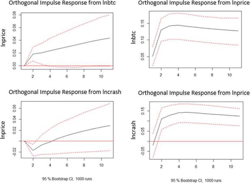
Based on Fig. 4, it is inferred that a 100% shock on lnbtc generates an increasing im-
pulse response at lnprice, being around 2% in the second week, a result similar to that
was obtained by Kristoufek (2013). A 100% boost of lncrash, in turn, causes a response
negative around 2% in the price in the first 2 weeks. A shock at 100% indicates a posi-
tive response for lnbtc and lncrash, reaching about 15% in the third week.
The histogram of the residuals of the model shows a concentration of the near zero ob-
servations with progressive reduction of the frequency along the tails. In order to verify
the existence of serial correlation in the residuals of the model, the tests of Portmanteau
(2006) (PT) and Breusch (1978) & Godfrey (1978) were applied. The test results showed
that the null hypothesis of no serial correlation cannot be rejected at the significance level
of 5%. For stability analysis of the model, the eigen values were obtained and they are con-
tained within the unit circle, confirming the stability of the model.
Table 5 Determination of the coefficient of each variable of VECM regressions
Variable Δlnpreçot(1) Δlnbtct(2) Δlncrasht(3)
Coef. Pr(>|t|) Coef. Pr(>|t|) Coef. Pr(>|t|)
α1 − 0.03* 0.021 0.09*** 0.000 − 0.06 0.191
α2 − 0.02 0.483 0.09. 0.061 − 0.60*** 0.000
crisis 0.09* 0.043 0.10 0.215 0.15 0.373
Δlnpricet-1 0.34*** 0.000 0.92*** 0.000 0.96*** 0.000
Δlncrasht-1 −0.06** 0.001 − 0.07. 0.064 − 0.19* 0.019
Δlnbtct-1 0.07. 0.061 −0.05 0.475 − 0.01 0.944
constant 0.09** 0.004 −0.27*** 0.000 −0.25* 0.050
significance level: ‘***’ 0.001 ‘**’ 0.01 ‘*’ 0.05 ‘.’ 0.1 ‘’ 1
(1) Adj. R2 = 27.07% (2) Adj. R2 = 20.43% (3) Adj. R2 = 34.18%Hakim das Neves Financial Innovation (2020) 6:21 Page 15 of 18
Table 6 Granger causality test
Null hypothesis (Ho) F Test P-value
X2 does not Granger-cause X1 14.79 0.0000
X1 does not Granger-cause X2 7.43 0.0000
Analysis by currency
The procedure applied to BCX can be replicated to local prices specified by each sover-
eign currency. The objective is to check if prices traded in different currencies are also
influenced by the structure of the global variables previously established. Only price ob-
servations are altered, which will be denominated in each respective currency. The ex-
pectation is that world events consistently impact the price at local brokerages.
Table 7 presents the coefficients of the cointegration matrix β1 and β2 of the error
correction term by sovereign currency. The analysis by sovereign currency reiterates
the behavior of the global analysis; it means that an increase of lnbtct-1, unaccompanied
in the same proportion by lnpricet-1 and lncrasht-1, brings a pressure on Δlnpricet, so
that in the following period the price variation also increases, considering that α1 and
α2 have a negative sign (Table 8).
On the other hand, a sudden increase of lncrasht-1 generates a positive error which,
when multiplied by α2, generates a decrease of Δ lnprice.
The coefficients for the variable Δlnbtct-1 in the equation Δlnpricet are positive for all
currencies and are significant at the level of 5% for six of twelve. The coefficients for
the variable Δlncrasht-1 are also significant at the 5% level for nine of twelve and, as ex-
pected, are all negative.
Fig. 4 Graph of the impulse-response functions for variables lnprice, lnbtc and lncrashHakim das Neves Financial Innovation (2020) 6:21 Page 16 of 18
Table 7 Coefficients of the cointegration matrix (β) of the error correction term by sovereign
currency
The coefficient of the dummy variable crisis is significant at the level of 5% for eight
currencies and positive for all of them; that is, there is strong and recurrent evidence
that the Bitcoin price traded in other sovereign currencies follows the trend and also
increases when there is an increase in the search for the term crisis in the world.
Conclusions
It is possible to identify a strong relationship, in the short and long term, between the
terms in Google searches and the Bitcoin price. The cointegration test of the curves
performed describes a tendency of simultaneous growth or decline between them. The
estimated VEC model confirms the long-term dynamics based not only on the global
analysis, but on a more detailed analysis of prices negotiated in different sovereign
currencies.
The result of the VEC model and the significance of the coefficients demonstrate that
the increase in Bitcoin interest, as measured by the number of searches for the keyword
bitcoin (bitcoin crash), is followed by an increase (fall) of Bitcoin price. The bidirec-
tional relationship exists and demonstrates that price Granger-causes the behavior of
lnbtc and lncrash, intensifying the understanding that there is a speculative driver in
Bitcoin’s transactions.
This research is based on previous studies that used the same methodology and simi-
lar variables of attractiveness. It is worth mentioning that a longer and more recent
period of data was added, confirming the cointegration between Google Trends attract-
iveness data and the Bitcoin price, a hypothesis that was not confirmed initially in
Table 8 Coefficients of Δprice equation per sovereign currency
Significance level: ‘***’ 0.001 ‘**’ 0.01 ‘*’ 0.05 ‘.’ 0.1 ‘’ 1Hakim das Neves Financial Innovation (2020) 6:21 Page 17 of 18
Kristoufek’s study (2013), which took into account a historical database between May
2011 and June 2013.
The crisis variable is useful for investment decision-making. In times of high demand
for news about a world economic crisis, there is an increase in the Bitcoin price, which
may be related to a greater demand for the virtual currency and its characteristics that
are favorable to these moments, such as low probability of being confiscated, high se-
curity, and high portability that allows bitcoins to be transferred globally in minutes.
Bitcoins priced in different sovereign currencies follow global price behavior and are
quickly adjusted by changing interest in currencies around the world and by crisis
events.
The findings may show to policymakers and monetary authorities that society is
afraid about losing their purchasing power in period of crisis, so people are looking for
buying safe haven assets, and Bitcoin might be one of them. Understanding these inter-
ests is fundamental to investors, who want to diversify their portfolio, and to govern-
ments, which can establish alternatives to avoid having their currencies depreciated
against Bitcoin.
Abbreviations
ADF: Augmented Dickey Fuller Test; AIC: Akaike Information Criterion; AUD: Australian Dollar; BCX: Bitcoin.com
Composite Price Index; BG: Breusch-Godfrey; BRL: Brazilian Real; BTC: Bitcoin; CAD: Canadian Dollar; CEO: Chief
Executive Officer; CNY: Yuan Renminbi; CPI: Consumer Price Index; DJIA: Dow Jones Industrial Average; EUR: Euro;
FFR: Federal Funds Rate; FPE: Final Prediction Error; FTSE: Financial Times Stock Exchange; GBP: Pound Sterling;
GP: Gold Price; HQ: Hannan-Quinn; IDR: Indonesian Rupiah; IMF: International Monetary Fund; JPY: Japanese yen;
KRW: South Korean Won; PLN: Polish Zloty; PT: Portmanteau; RUB: Russian Ruble; SC: Schwarz; USA: United States of
America; USD: United States Dollar; USDI: US Dollar Index; VAR: Vector Autoregressive; VEC: Vector Error Correction;
VECM: Vector Error Correction Model
Acknowledgements
My advisor, Professor Ricardo Masini, helped and gave me the support to guarantee the technical quality of this
research.
Authors’ contributions
The author(s) read and approved the final manuscript.
Funding
I know of no conflicts of interest associated with this publication, and there has been no financial support for this
work that could have influenced its outcome. There is no conflict of competing interests.
Availability of data and materials
The selected database to be considered by the model was found in three electronic data sources: Google Trends
(https://trends.google.com/trends/), Bitcoincharts (https://bitcoincharts.com/charts/) and Bitcoin.com (https://charts.
bitcoin.com/btc/chart/price). The period studied is the weeks between December 17, 2012 and February 12, 2018. The
database starts in December 2012 due to a technical limitation of Google Trends; until that date, the tool produced
weekly observations, while the extended period generates monthly observations.
Competing interests
The authors declare that they have no competing interests.
Received: 17 April 2019 Accepted: 11 February 2020
References
Akaike H (1969) Fitting autoregressive models for prediction. Ann Inst Stat Math 21:243–247
Al-Khazali O, Bouri E, Roubaud D (2018) The impact of positive and negative macroeconomic news surprises: gold versus
Bitcoin. Econ Bull, AccessEcon 38:373–382
Bacen. Comunicado n° 31.379, de 16 de novembro de 2017. Alerta sobre os riscos decorrentes de operações de guarda e
negociação das denominadas moedas virtuais. http://www.bcb.gov.br/pre/normativos/busca/normativo.asp?numero=313
79&tipo=Comunicado&data=16/11/2017, visited on 7 May 2018
Balcilar M et al (2017) Can volume predict bitcoin returns and volatility? A quantiles-based approach. Econ Model https://ssrn.
com/abstract=2938555, visited on 12 Dec 2017
Bitcoin.com. Bitcoin core (BTC) price. https://charts.bitcoin.com/btc/chart/price, visited on 1 March 2018Hakim das Neves Financial Innovation (2020) 6:21 Page 18 of 18
Bitcoincharts. Pricechart. https://bitcoincharts.com/charts/bitstampUSD#rg60ztgSzm1g10zm2g25zv, visited on 1 March 2018
Bouoiyour J, Selmi R (2015) What does bitcoin look like? Ann Econ Financ 16:449–492
Bouri E, Gil-Alana L, Gupta R, Roubaud D (2018) Modelling long memory volatility in the Bitcoin market: evidence of
persistence and structural breaks. Int J Finance Econ
Bouri E et al (2017) Bitcoin for energy commodities before and after the December 2013 crash: diversifier, hedge or safe
haven? Appl Econ https://ssrn.com/abstract=2925783, visited on 20 Dec 2017
Breusch TS (1978) Testing for autocorrelation in dynamic linear models. Aust Econ Pap 17:334–355
Buchholz M, Delaney J, Warren J, Parker J (2012) Bits and bets, information, price volatility, and demand for bitcoin.
Economics 312
Bueno RLS (2015) Econometria de séries temporais. Cengage Learning, Sao Paulo
Buterin V (2013) The bitcoin crash: an examination. Bitcoin Magazine, Nashville https://bitcoinmagazine.com/articles/the-
bitcoin-crash-an-examination-1365911041/, visited on 3 June 2018
Chao X, Kou G, Peng Y, Alsaadi FE (2019) Behavior monitoring methods for trade-based money laundering integrating macro
and micro prudential regulation: a case from China. Technol Econ Dev Econ 25(6):1081–1096
Ciaian P, Miroslava R, Kancs D (2016a) Can bitcoin become a global currency? IseB 14:883–919
Ciaian P, Miroslava R, Kancs D (2016b) The economics of bitcoin price formation. Appl Econ 48:1799–1815
Civitarese JM (2018) Does metcalfe’s law explain bitcoin prices? A time series analysis. SSRN Electronic Journal
Davies DC (2014) The curious case of bitcoin: is bitcoin volatility driven by online search? University of Victoria, Victoria
Dyhrberg AH (2016) Hedging capabilities of bitcoin. Is it the virtual gold? Financ Res Lett 16:139–144
Engle RF, Granger CWJ (1987) Co-integration and error correction: representation, estimation and testing. Econometrica 55:
251–276
G1. Crise da Grécia: veja perguntas e respostas e o que acontece agora. http://g1.globo.com/economia/noticia/2015/07/crise-
da-grecia-veja-perguntas-e-respostas-e-o-que-acontece-agora.html, visited on 22 June 2018
Gandal N et al (2018) Price manipulation in the bitcoin ecosystem. J Monet Econ 95:86–96
Godfrey LG (1978) Testing for higher order serial correlation in regression equations when the regressors include lagged
dependent variables. Econometrica 46:1303–1313
Google Trends. https://trends.google.com/trends/?geo=US, visited on 1 Mar 2018
Hannan E, Quinn B (1979) The determination of the order of an autoregression. J R Stat Soc:190–195
Hayes A (2017) Cryptocurrency value formation: an empirical analysis leading to a cost of production model for valuing
bitcoin. Telematics Inform. https://doi.org/10.2139/ssrn.2648366 visited on 25 Jan 2018
Johansen S (1988) Statistical analysis of Cointegrating vectors. J Econ Dyn Control 12:231–254
Kwan C. How the Greece debt crisis showed the world that bitcoin is a store of value. https://cointelegraph.com/news/how-
the-greece-debt-crisis-showed-the-worldthat-bitcoin-is-a-store-of-value, visited on 22 June 2018.
Kelion L Bitcoin sinks after China restricts yuan exchanges. http://www.bbc.com/news/technology-25428866, visited on 3
June 2018
Kim YB et al (2017) When bitcoin encounters information in an online forum: using text mining to analyse user opinions and
predict value fluctuation. PLoS ONE 12
Kristoufek L (2013) Bitcoin meets google trends and wikipedia: quantifying the relationship between phenomena of the
Internet era. Sci Rep 3
Kristoufek L (2015) What are the main drivers of the bitcoin price? Evidence from wavelet coherence analysis. PLoS ONE
Nakamoto, S. (2008) Bitcoin: a peer-to-peer electronic cash system. https://bitcoin.org/bitcoin.pdf , visited on 15 Oct 2017
Nasir M, Huynh D, Nguyen P, Duong D (2019) Forecasting cryptocurrency returns and volume using search engines. Financ Innov
Pagliery J Greeks are rushing to bitcoin. http://money.cnn.com/2015/06/29/technology/greece-bitcoin/index.html, visited on
22 June 2018
Pfaff B (2006) Analysis of integrated and Cointegrated time series with R. Springer, NY
Polasik M et al (2015) Price fluctuations and the use of Bitcoin: an empirical inquiry. Int J Eletron Commerce 20:9–49
Reuters. China bans banks from bitcoin transactions. https://www.smh.com.au/business/markets/china-bans-banks-from-
bitcoin-transactions-20131206-2yugy.html, visited on 3 June 2018
Rosenfeld E Greek crisis stokes bitcoin prices higher. https://www.cnbc.com/2015/06/29/greek-crisis-stokes-bitcoin-prices-
higher.html, visited on 22 June 2018
S Kumar A, Ajaz T (2019) Co-movement in crypto-currency markets: evidences from wavelet analysis. Financ Innov 5:33.
https://doi.org/10.1186/s40854-019-0143-3
Schwarz G (1978) Estimating the dimension of a model. Ann Stat 6:461–464
Van Wijk D (2013) What can be expected from the BitCoin? Erasmus Rotterdam Universiteit, Rotterdam
Wooldridge JM (2006) Introdução à Econometria - uma abordagem moderna. Thomson
Xu M, Chen X, Kou G (2019) A systematic review of blockchain. Financ Innov 5:27. https://doi.org/10.1186/s40854-019-0147-z
Yermack D (2015) Is bitcoin a real currency? An economic appraisal, pp 31–43
Zhu Y, Dickinson D, Li J (2017) Analysis on the influence factors of Bitcoin’s price based on VEC model. Financ Innov
Publisher’s Note
Springer Nature remains neutral with regard to jurisdictional claims in published maps and institutional affiliations.You can also read