Dynamic Automaton-Guided Reward Shaping for Monte Carlo Tree Search
←
→
Page content transcription
If your browser does not render page correctly, please read the page content below
The Thirty-Fifth AAAI Conference on Artificial Intelligence (AAAI-21)

     Dynamic Automaton-Guided Reward Shaping for Monte Carlo Tree Search
  Alvaro Velasquez1 , Brett Bissey2 , Lior Barak2 , Andre Beckus1 , Ismail Alkhouri2 , Daniel Melcer3 ,
                                              George Atia2
                                    1
                                      Information Directorate, Air Force Research Laboratory
                         2
                       Department of Electrical and Computer Engineering, University of Central Florida
                                  3
                                    Department of Computer Science, Northeastern University
          {alvaro.velasquez.1, andre.beckus}@us.af.mil, {brettbissey, lior.barak, ialkhouri}@knights.ucf.edu,
                                         melcer.d@northeastern.edu, george.atia@ucf.edu
                             Abstract                                            Given an automaton representation of the underlying
                                                                              agent objective, we investigate how to guide and acceler-
  Reinforcement learning and planning have been revolution-                   ate the derivation of decision-making policies by leverag-
  ized in recent years, due in part to the mass adoption of deep
  convolutional neural networks and the resurgence of pow-
                                                                              ing this structured representation. This use of automata al-
  erful methods to refine decision-making policies. However,                  lows us to reason about non-Markovian reward signals that
  the problem of sparse reward signals and their representation               account for the prior state history of the agent, which is
  remains pervasive in many domains. While various reward-                    useful and sometimes necessary in domains with sparse re-
  shaping mechanisms and imitation learning approaches have                   wards or partial observability (Toro Icarte et al. 2019). In
  been proposed to mitigate this problem, the use of human-                   particular, we make two main contributions. First, we in-
  aided artificial rewards introduces human error, sub-optimal                troduce Automaton-Guided Reward Shaping (AGRS) for
  behavior, and a greater propensity for reward hacking. In this              Monte Carlo Tree Search (MCTS) algorithms as a means to
  paper, we mitigate this by representing objectives as automata              mitigate the sparse rewards problem by leveraging the em-
  in order to define novel reward shaping functions over this                 pirical expected value of transitions within the automaton
  structured representation. In doing so, we address the sparse
  rewards problem within a novel implementation of Monte
                                                                              representation of the underlying objective. In this sense, ex-
  Carlo Tree Search (MCTS) by proposing a reward shaping                      pected value denotes the frequency with which transitions
  function which is updated dynamically to capture statistics on              in the automaton have been observed as part of a trajec-
  the utility of each automaton transition as it pertains to satis-           tory which satisfies the given objective. We integrate the
  fying the goal of the agent. We further demonstrate that such               proposed AGRS within modern implementations of MCTS
  automaton-guided reward shaping can be utilized to facili-                  that utilize deep reinforcement learning to train Convolu-
  tate transfer learning between different environments when                  tional Neural Networks (CNNs) for policy prediction and
  the objective is the same.                                                  value estimation. Our second contribution entails the use of
                                                                              the aforementioned automata as a means to transfer learned
                                                                              information between two problem instances that share the
                        Introduction                                          same objective. In particular, we record the empirical ex-
In reinforcement learning and planning settings, a reward                     pected value of transitions in the objective automaton in a
signal over state-action pairs is used to reinforce and deter                 simple environment and use these to bootstrap the learning
positive and negative action outcomes, respectively. How-                     process in a similar, more complex environment. We demon-
ever, from a practical perspective, it is common to have a                    strate the effectiveness of AGRS within MCTS, henceforth
high-level objective which can be captured as a language                      referred to as MCTSA , by comparing the win-rate curves to
of what would constitute good behaviors. Such objectives                      those of a vanilla MCTS baseline on randomized grid-world
can be represented via various types of automata. For ex-                     problems.
ample, the deterministic finite automata we consider in this                     The foregoing is useful as a complement to existing ap-
paper can represent any regular language and thus afford a                    proaches by reasoning over both the learned representation
large space of possibilities for defining objectives. If these                of agent-environment dynamics through deep CNNs as well
objectives are expressed in natural language, there are trans-                as the learned representation of the underlying objective via
lation mechanisms for obtaining the corresponding automa-                     automata. We argue that this is particularly useful due to
ton (Brunello, Montanari, and Reynolds 2019). On the other                    the typically low dimensionality of the automaton that rep-
hand, there are also approaches for learning the graph struc-                 resents the objective. This means that individual transitions
ture of the automaton that represents a given reward signal                   within the automaton correspond to potentially many differ-
(Xu et al. 2020; Gaon and Brafman 2020; Toro Icarte et al.                    ent transitions within the environment and, hence, within the
2019), so such approaches could be used to learn the au-                      Monte Carlo tree. Thus, reward shaping defined over the for-
tomaton structure from a reward signal.                                       mer can be used to accelerate learning over many instances
                                                                              of the latter.
Copyright © 2021, Association for the Advancement of Artificial
Intelligence (www.aaai.org). All rights reserved.

                                                                      12015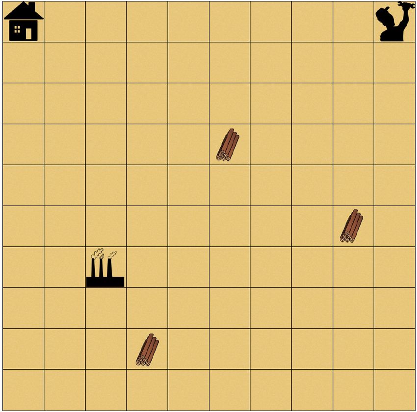
Preliminaries                                                                                               ¬wood   ω0         ¬factory∧wood
We assume that the agent-environment dynamics are mod-                                                                    factory∧wood

eled by a Non-Markovian Reward Decision Process (NM-                                                          factory∨¬wood   ω1
                                                                                                                                           factory
RDP), defined below.
Definition 1 (Non-Markovian Reward Decision Process)                                                              ¬factory∧wood            ω2
                                                                                                                                                     ¬factory
A Non-Markovian Reward Decision Process (NMRDP) is a
non-deterministic probabilistic process represented by the
tuple M = (S, s0 , A, T, R), where S is a set of states, s0                  Figure 1: (left) NMRDP consisting of four states
is the initial state, A is a set of actions, T (s0 |s, a) ∈ [0, 1]           s0 , s1 , s2 , s3 denoting which tile the agent is on, starting
denotes the probability of transitioning from state s to state               with s0 in the top-right corner and progressing counter-
s0 when action a is taken, and R : S ∗ → R is a reward                       clockwise. There are four actions a1 , a2 , a3 , a4 correspond-
observed for a given trajectory of states. We denote by                      ing to LEFT, DOWN, RIGHT, UP. The transition func-
S ∗ the set of possible state sequences and A(s) ⊆ A the                     tion is deterministic and defined in the obvious way (e.g.
actions available in s.                                                      T (s1 |s0 , a1 ) = 1). Given a set of atomic propositions AP =
                                                                             {wood, factory, house}, we have the following state labels:
   Note that the definition of NMRDP closely resembles that                  L(s0 ) = {}, L(s1 ) = {wood}, L(s2 ) = {house}, L(s3 ) =
of a Markov Decision Process (MDP). However, the non-                        {factory}. That is, the labels correspond to the atomic propo-
Markovian reward formulation R : S ∗ → R (often denoted                      sitions that are true in a given state. (right) Automaton
by R : (S × A)∗ × S → R in the literature) depends on
                                                                             A = (Ω = {ω0 , ω1 , ω2 }, ω0 , Σ = 2{wood, factory, house} , δ =
the history of agent behavior. Given an NMRDP, we define                            ¬wood
a labeling function L : S → 2AP that maps a state in the                     {ω0 −−−−→ ω0 , . . . }, F = {ω1 }) corresponding to the ob-
NMRDP to a set of atomic propositions in AP which hold                       jective that the agent will eventually be on a tile containing
for that given state. We illustrate this with a simple example               wood and that, if the agent stands on said tile, then it must
in Figure 1 (left). The atomic propositions AP assigned to                   eventually reach a tile containing a factory. Transitions visu-
the NMRDP can correspond to salient features of the state                    alized with a Boolean formula are used as a shorthand nota-
space and will be used to define the transition dynamics of                  tion for the sets of atomic propositions that cause that transi-
                                                                                                                          ¬f ∧w
the objective automaton as defined below.                                    tion. For example, the transition ω0 −−−−→ ω2 (f for factory
Definition 2 (Automaton) An automaton is a tuple A =                         and w for wood) in the automaton is shorthand for transi-
(Ω, ω0 , Σ, δ, F ), where Ω is the set of nodes with initial node            tions (ω0 , σ, ω2 ) ∈ δ such that factory ∈
                                                                                                                       / σ and wood ∈ σ.
ω0 ∈ Ω, Σ = 2AP is an alphabet defined over a given set
of atomic propositions AP , δ : Ω × Σ → Ω is the transition
function, and F ⊆ Ω is the set of accepting nodes. For sim-                  π(s0 ) = a1 (Go LEFT), π(s1 ) = a2 (Go DOWN), π(s2 ) =
plicity, we use ω −
                     σ
                     → ω 0 ∈ δ to denote that σ ∈ Σ causes a                 a3 (Go RIGHT), π(s3 ) = · (no-op) yields a finite trajectory
transition from node ω to ω 0 .                                              of four states (s0 , s1 , s2 , s3 ) whose corresponding trace in
                                                                                                     L(s0 )         L(s1 )           L(s2 )                L(s3 )
    Given an automaton A = (Ω, ω0 , Σ, δ, F ), a trace is de-                the automaton is ω0 −−−→ ω0 −−−→ ω2 −−−→ ω2 −−−→
                                    σi 1      σi 2      σi 3                 ω1 , where L(s0 ) = {}, L(s1 ) = {wood}, L(s2 ) =
fined as a sequence of nodes ω0 −−→      ωi1 −−→   ωi2 −−→   ...             {house}, L(s3 ) = {factory}. Since ω1 ∈ F , this policy
starting in the initial node ω0 such that, for each transition,              leads to a trajectory in the NMRDP which satisfies the ob-
we have (ωik , σik , ωik+1 ) ∈ δ. An accepting trace is one                  jective. In order to reinforce such behavior and formalize
which ends in some node belonging to the accepting set F .                   the foregoing, we utilize a binary reward signal for the
Such a trace is said to satisfy the objective being represented              NMRDP denoting whether the underlying automaton ob-
by the automaton. For the remainder of this paper, we use                    jective has been satisfied by an observed trajectory ~s =
the terms nodes and states to refer to vertices in automata                  (s0 , . . . , st , st+1 ). Let tr : S ∗ → Ω∗ and last : Ω∗ 7→ Ω
and NMRDPs, respectively.                                                    denote the mapping of a given trajectory to its correspond-
    Until now, we have used the notion of an atomic propo-                   ing trace and the last node in a trace, respectively. A trace ω  ~
sition set AP in defining the labeling function of an NM-                    is accepting if and only if last(~      ω ) ∈ F . The reward signal
RDP and the alphabet of an automaton. In this paper, our                     R : S ∗ → {0, 1} is defined in Equation (1) below.
focus is on deriving a policy for a given NMRDP such that
it is conducive to satisfying a given objective by leveraging

                                                                                                             1 last(tr(~s)) ∈ F
the automaton representation of the same, where both the                                         R(~s) =                                     (1)
                                                                                                             0 otherwise
NMRDP and the automaton share the same set of atomic
propositions AP . As a result, an arbitrary transition from                     Note that the use of such a reward signal makes the prob-
state s to s0 in the NMRDP can cause a transition in the                     lem of finding optimal policies susceptible to sparse re-
automaton objective via the observance of atomic proposi-                    wards. Indeed, one can envision many instances where such
tions that hold in s0 as determined by the NMRDP labeling                    a reward is only accessible after a long time horizon, which
function L. To illustrate the relationship between trajecto-                 can hinder learning. The proposed AGRS will mitigate this
ries, or sequences of states, in an NMRDP and their cor-                     problem by providing artificial intermediate rewards that re-
responding traces, or sequences of nodes, in the automa-                     flect the frequency with which transitions in the automaton
ton, recall the example in Figure 1. Note that the policy                    objective have been conducive to satisfying the objective.

                                                                     12016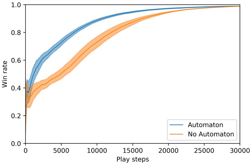
a∧b
Finite-Trace Linear Temporal Logic (LTLf )
                                                                                                ¬a∧¬b                 ¬b         1
A classic problem in formal methods is that of convert-
ing a high-level behavioral specification, or objective, into                                    ω2       a∧¬b        ω1   b     ω0
a form that is amenable to mathematical reasoning. Indeed,
                                                                                                          ¬a∧b
the foregoing discussion on utilizing automata representa-                                                                  a
                                                                                                                      ¬a
tions of objectives subsumes the idea that we have some
means of performing this translation from objective to au-                                                            ω3
tomaton. There are various ways to mitigate this problem by
enforcing that the given objective be specified in some for-                                        ω2
                                                                                            ¬b              1                             1
mal logic which can then be easily converted into an equiv-                                                                1
                                                                                    ω4                               ω1         ω0
alent automaton. In order to represent the objective of an                                  b               ¬b                        a
                                                                                                    ω3                     b              ω5
agent as an automaton, we choose the formal logic known
as finite-trace Linear Temporal Logic (LTLf ) for its simple
syntax and semantics. This logic is known to have an equiv-
alent automaton representation (De Giacomo, De Masellis,                                 Figure 2: Simple example automata.
and Montali 2014; De Giacomo and Vardi 2015; Camacho
et al. 2018a). Other choices include finite-trace Linear Dy-               ton. Furthermore, optimal policy invariance (Ng, Harada,
namic Logic (LDLf ) and regular expressions.                               and Russell 1999) can be established for tabular settings.
   Given a set of atomic propositions AP , a formula in LTLf
is constructed inductively using the operations p, ¬φ, φ1 ∨                Definition 3 (Reward Machine) A reward machine is an
φ2 , Xφ, Fφ, Gφ, φ1 Uφ2 , where p ∈ AP and φ, φ1 , φ2 are                  automaton given by the tuple A = (Ω, ω0 , Σ, δ, R, ρ), where
LTLf formulas. The operators ¬, ∨ denote logical negation                  Ω is the set of nodes with initial node ω0 ∈ Ω, Σ = 2AP is
and disjunction and X, F, G, U denote the Next, Eventu-                    an alphabet defined over a given set of atomic propositions
ally, Always, and Until operators, respectively, such that Xφ              AP , δ : Ω × Σ → Ω is the transition function, R is an
(resp. Fφ, Gφ, φ1 Uφ) holds iff φ holds in the next time step              output alphabet denoting the possible reward values, and
(resp. some time in the future, all times in the future, at some           ρ : Ω × Σ → R is the output function.
point and φ1 is true until that point). An example LTLf for-                  Consider the reward shaping function obtained from per-
mula is (F wood) ∧ (F wood =⇒ F factory), which cor-                       forming value iteration over a reward machine representa-
responds to the automaton objective of Figure 1 (right).                   tion of the objective given by the formula φ = (Fa) ∧ (Fb),
   For the remainder of this paper, we will use the automa-                whose automaton is given in Figure 2 (top). The reward ma-
ton A of a given LTLf objective to define a reward-shaping                 chine has R = {0, 1} with a reward value of 1 being ob-
function reflecting the frequency with which individual tran-              served if φ is satisfied. This yields the output transition val-
sitions in A were part of some accepting trace. In particu-                ues of ρ(ω2 , a ∧ b) = ρ(ω1 , b) = ρ(ω3 , a) = 1 and ρ = 0 for
lar, we integrate this reward-shaping function within MCTS                 all other transitions. Consider value iteration over the func-
in order to leverage the power of modern MCTS solvers                      tion below as proposed in (Camacho et al. 2019), where ini-
and exploit their lookahead property to simulaneously look                 tial values are set to 0.
ahead in the NMRDP and the automaton objective.                                          V (ω) :=        max        ρ(ω, σ) + γV (ω 0 )        (2)
                                                                                                      ω 0 =δ(ω,σ)
                      Related Work                                            Due to the symmetry of traces ω2 → ω1 → ω0 and
Given an infinite-trace LTL objective, reinforcement learn-                ω2 → ω3 → ω0 , the same values would be obtained for each
ing has been applied to learn controllers using temporal dif-              of those corresponding transitions, which may be an uninfor-
ference learning (Sadigh et al. 2014), value iteration (Hasan-             mative reward shaping mechanism in some settings. Indeed,
beig, Abate, and Kroening 2018), neural fitted Q-learning                  one can envision arbitrary environments where observing a
(Hasanbeig, Abate, and Kroening 2019), and traditional Q-                  followed by b may be much more efficient than observing b
learning (Hahn et al. 2019). These approaches reward the                   followed by a. However, this type of reward shaping would
agent for reaching an accepting component of the automa-                   not exploit such knowledge.
ton, but they do not yield intermediate rewards to mitigate                   Another approach using automata for reward shaping was
the sparse rewards problem.                                                proposed in (Camacho et al. 2017, 2018b), where instead of
   More related to our approach is the use of reward ma-                   solving a planning problem over a reward machine, reward
chines (Icarte et al. 2018) as described in Definition 3. These            shaping is defined over each automaton transition to be in-
correspond to automata-based representations of the reward                 versely proportional to the distance between a given node
function. By treating these reward machines as a form of ab-               and an accepting node in the automaton of an LTL objective.
stract NMRDP, reward shaping functions have been defined                   Like the previous example, this introduces some uninforma-
in the literature (Icarte et al. 2018; Camacho et al. 2019).               tive and potentially unproductive rewards. Indeed, consider
In particular, note that the nodes and transitions of such au-             the LTL objective given by φ = (XXXa) ∨ (b ∧ Xb) whose
tomata can be treated as states and actions in Q-learning and              automaton is shown in Figure 2 (bottom).
value iteration approaches. Such methods have been pro-                       Note that the aforementioned reward shaping will favor
                                                                                          b          b
posed and yield a value for each transition in the automa-                 transitions ω4 →
                                                                                          − ω3 , ω 3 →
                                                                                                     − ω5 in the automaton over transi-

                                                                   12017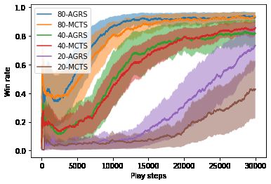
¬b          ¬b
tions ω4 −→ ω2 , ω3 −→ ω1 since the distance to accepting                φ whose automaton is defined by A = (Ω, ω0 , Σ, δ, F ). As
node ω5 is greater for the latter. However, again we can en-             such, we must establish a connection between the agent-
vision scenarios where rewards defined in this way are unin-             environment dynamics defined by M and the environment-
formative. For example, consider an NMRDP where a node                                                                   L(s)
                                                                         objective dynamics defined by A. Let ω −−−→ ω 0 denote
labeled a is three steps away from the initial state, but the            that the observance of labels, or features, L(s) (e.g., “safe”,
second observance of b is many steps away.                               “hostile”, etc.) of state s (e.g., an image) in any trajectory
   In contrast, we focus on a dynamic reward shaping func-               of M causes a transition from ω to ω 0 in A (see Figure 1
tion that changes based on observed experience in that each              for an example). This establishes a connection between the
transition value in the automaton captures the empirical ex-             NMRDP M and the automaton A. In particular, note that
pected value associated with said transition. This is based              any trajectory of states S~ = (s0 , . . . , st ) in M has a corre-
on the experience collected by the agent, thereby implic-                                 ~
itly reflecting knowledge about the given environment in a               sponding trace Ω = (ω0 , . . . , ωt ) in A.
way that the more static reward shaping mechanisms pre-                     MCTS functions by (a) simulating experience from a
viously mentioned cannot. MCTS lends itself well for the                 given state st by looking ahead in M and (b) selecting an
adoption of such an approach given that each search tree is              action to take in st based on predicted action values from
the culmination of many trajectories in the NMRDP and its                the simulated experience (see Algorithm 1). For (a), a search
corresponding traces in the automaton objective. Thus, tree              tree is expanded by selecting actions according to the tree
search provides a natural way to refine the estimated val-               policy (3) starting from the root st until a leaf in the tree is
ues of each automaton transition via simulated experience                encountered (Lines 7 through 12). The tree policy consists
before the agent makes a real decision in the environment.               of an action value function Q and an exploration function
In particular, the lookahead property of MCTS naturally al-              U as formulated in modern MCTS implementations (Silver
lows the same within a given objective automaton. We ex-                 et al. 2017), where cUCB is a constant used to control the
ploit this lookahead in the proposed AGRS function and ap-               influence of exploration. The Y function in (3) corresponds
ply it within a modern MCTS implementation using deep                    to the proposed AGRS function discussed later in this sec-
CNNs similar to those proposed for the game of Go (Silver                tion. Once an action is taken in a leaf state (Line 13), a new
et al. 2016) (Silver et al. 2017), various other board games             state is observed (Line 14) in the form of a newly added leaf
(Silver et al. 2018) (Anthony, Tian, and Barber 2017), and               sexpand . The value VCNN (sexpand ) of this new leaf as well as
Atari (Schrittwieser et al. 2020).                                       its predicted action probabilities πCNN (a|sexpand ) are given
   We also explore the use of our proposed AGRS as a trans-              by the CNN of the agent (Line 15). This is known as the Ex-
fer learning mechanism. Despite the tremendous success of                pansion phase of MCTS. After expansion, the Update phase
transfer learning in fields like natural language processing             begins, wherein the values of the edges (s, a) corresponding
(Devlin et al. 2018) and computer vision (Weiss, Khosh-                  to actions on the path leading from the root st to the new leaf
goftaar, and Wang 2016), transfer learning in the fields of              node sexpand are updated (Lines 18 through 21). These values
reinforcement learning and planning faces additional chal-               are {N (s, a), W (s, a), Q(s, a), πCNN (a|s)}, where N (s, a)
lenges due in part to the temporally extended objectives of              denotes the number of times action a has been taken in
the agents and the fact that actions taken by these agents can           state s in the search tree, W (s, a) is the total cumulative
affect the probability distribution of future events. The area           value derived from VCNN (s0 ) for all leafs s0 that were even-
of curriculum learning (Narvekar et al. 2020) addresses this             tually expanded when action a was taken in state s, and
by decomposing the learning task into a graph of sub-tasks               Q(s, a) = W (s, a)/N (s, a) is the action value function
and bootstrapping the learning process over these first. For             yielding the empirical expected values of actions in a given
example, this may include learning chess by first ignoring all           state. After this Update phase, a new iteration begins at the
pawns and other pieces, and progressively adding more com-               root of the tree. The tree expansion and update process re-
plexity as the agent learns good policies. State and action              peats until a user-defined limit on the number of expansions
mappings or embeddings have also been explored for han-                  is reached (Line 2). After this process of simulating expe-
dling transfer between different environments (Taylor and                rience (a) is done, (b) is achieved by taking an action in
Stone 2009; Chen et al. 2019). These can also be used to                 the real world at the root st of theP    tree according to the
derive similarity metrics between the state spaces of dif-               play policy πplay (a|st ) ∝ N (st , a)/ b N (st , b) (Line 22)
ferent environments. In this paper, we avoid the standard                as used in (Silver et al. 2016) due to lowered outlier sensi-
modus operandi of focusing on state spaces or neural net-                tivity when compared to a play policy that maximizes ac-
work weights to enable transfer learning and instead focus               tion value (Enzenberger et al. 2010). The foregoing corre-
on commonality found in the underlying goals of the agent                sponds to a single call of the lookahead process given by
as given by their automaton representation.                              Algorithm 1. Algorithm 2 utilizes multiple lookahead calls
                                                                         in sequence in order to solve the given NMRDP by taking
        Monte Carlo Tree Search with                                     actions in sequence using the play policy returned by Algo-
                                                                         rithm 1 and using the data generated from these transitions
      Automaton-Guided Reward Shaping                                    to update the CNN of the agent. Indeed, using Algorithm 2
For the purposes of the MCTSA algorithm, we are in-                      as a reference, note that once an action is taken using the
terested in finding a policy for a given NMRDP M =                       play policy (Line 9), a new state st+1 is observed (Line 10)
(S, s0 , A, T, R) which satisfies a given LTLf specification             and the process begins again with st+1 at the root of a new

                                                                 12018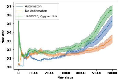
tree. Samples of the form (st , πplay (·|st ), r, st+1 ) are derived                Algorithm 1: LookaheadA
from such actions following the play policy πplay and are                           begin
stored (Line 14) in order to train the CNN (Line 21), where                            Input: NMRDP M, state s, Automaton A, node
r = R((s0 , . . . , st+1 ), πplay (·|st )) denotes the reward ob-                       ω, NN fθ
served. As defined in equation (1), we have r = 1 iff the                       1      W (s, a), N (s, a), Q(s, a) := 0
trajectory corresponding to the sequence of states from s0                      2      for k := 1 to expansionLimit do
to st+1 yields a satisfying trace in the given automaton ob-                    3          t := 0
jective (see Definition 2) and r = 0 otherwise. The entire                      4          st := s
process can be repeated over many episodes (Line 3) until                       5          XM := ∅          // stores transitions
the performance of πplay converges.                                             6          ωt := δ(ω, L(st ))
                                                                                7          while st not a leaf node do
πtree (s, ω) = argmaxa∈A (Q(s, a) + U (s, a) + Y (s, a, ω))                     8               a ∼ πtree (st , ωt )        // selection
                                                               (3)              9               st+1 ∼ T (·|st , a)
                                                                                                ωt+1 := δ(ωtS   , L(st+1 ))
                                   qP
                                                                               10
                                      b∈A(s) N (s, b)                          11               XM := XM {(st , a, st+1 )}
        U (s, a) = cUCB πCNN (a|s)                             (4)
                                    1 + N (s, a)                               12               t := t + 1
                                                                             13          a ∼ πtree (st , ωt )             // selection
 Y (s, a, ω) = cA max VA (ω, ω 0 ) , 0max 0 Y (s0 , a0 , ω 0 )                 14          sexpand ∼ T (·|st , a)
                                         a ∈A(s )
                                                                (5)            15          (VCNN (sexpand ), πCNN (·|sexpand )) :=
                                                                                             fθ (sexpand )                  // expansion
   For the AGRS component, we define a reward shaping                          16          XM := XM {(st , a, sexpand )}
                                                                                                           S
function Y : S × A × Ω → [0, 1] which is used as                               17
                                                                               18          for Each (s, a, s0 ) in XM do
part of the tree policy in equation (3). The AGRS function                     19               W (s, a) := W (s, a) + V (sexpand )
Y (s, a, ω) given by equation (5) recursively finds the max-                   20               N (s, a) := N (s, a) + 1
imum automaton transition value anywhere in the subtree                        21               Q(s, a) := W (s, a)/N (s, a)
rooted at state s, where ω is the corresponding automaton                                         // update tree
node that the agent is currently in at state s and we have                     22      Return πplay (a|s)
T (s0 |s, a) > 0, (ω, L(s0 ), ω 0 ) ∈ δ. This automaton transi-
tion value is given by VA (ω, ω 0 ) = WA (ω, ω 0 )/NA (ω, ω 0 ),                    Algorithm 2: Monte-Carlo Tree Search with
where WA (ω, ω 0 ) denotes the number of times a transition                          Automaton-Guided Reward Shaping MCTSA
ω → ω 0 in the automaton has led to an accepting trace in the                       begin
automaton and NA (ω, ω 0 ) denotes the total number of times                           Input: NMRDP M, Automaton A, NN fθ
that transition has been observed. The constant cA is used to                   1      WA (ω, ω 0 ), NA (ω, ω 0 ), VA (ω, ω 0 ) := 0
control the influence of AGRS on the tree policy. Note that                     2      M em := ∅
these values are updated after every episode in Algorithm 2                     3      for each episode do
(Lines 16 through 19).                                                          4          t := 0
   We compare the foregoing proposed MCTSA approach                             5          st := s0
against a modern vanilla MCTS approach using two grid-                          6          ωt := δ(ω0 , L(s0 ))
world environments Blind Craftsman and Treasure Pit de-                         7          XA = ∅           // stores transitions
fined in the next section and visualized in Figure 3. In these                  8          while st is not terminal do
environments, an agent has 6 possible actions correspond-                       9              a ∼ LookaheadA (M, st , A, ωt , fθ )
ing to moves in any of the cardinal directions, an action to                   10              st+1 ∼ T (·|st , a)
interact with the environment, and no-op.                                      11              ωt+1 := δ(ωt , L(st+1 ))
                                                                               12              r ∼ R(st , a,Sst+1 )
                  Experimental Results                                         13              XA := XA {(ω        St , ωt+1 )}
                                                                               14              M em := M em {(st , a, r, st+1 )}
We evaluate MCTSA using 10 × 10 and 25 × 25 grid-world
                                                                               15              t := t + 1
environments defined in the sequel. For each instance of a
10 × 10 environment, the object layout of the grid-world is                    16          for Each (ω, ω 0 ) in XA do
randomly generated and remains the same for every episode.                     17              WA (ω, ω 0 ) :=
We compute the average performance and variance of 100                                           WA (ω, ω 0 ) + R(st−1 , a, st )
such instances using MCTSA and a vanilla MCTS baseline                         18              NA (ω, ω 0 ) := NA (ω, ω 0 ) + 1
that does not use the AGRS function Y (i.e., Y (s, a, ω) = 0,                  19              VA (ω, ω 0 ) := WA (ω, ω 0 )/NA (ω, ω 0 )
for all s, a, ω). Each instance is trained for 30,000 play steps,                                // update automaton stats
corresponding to a varying number of episodes per instance.                    20          Let (p, v) := fθ (s)
The 25 × 25 environments will be used in Section 6 to                          21          Train θ using loss
demonstrate the effectiveness of the AGRS function as a                                      E(s,a,r,s0 )∼M em (r − v)2 − aT log p
transfer learning mechanism from 10 × 10 to 25 × 25 in-
stances that share the same objective automaton.

                                                                       12019
The CNN used during the expansion phase of MCTSA to
obtain πCNN , VCNN consists of a shared trunk with separate
policy and value heads. The trunk contains four layers. The
first two are convolutional layers with a 5 × 5 kernel, 32 and
64 channels, respectively, and ELU activation. The next two
layers are fully connected with ReLU activation; the first is
of size 256 and the second of size 128. The value and pol-
icy head each contain a fully connected layer of size 128
with ReLU activation. The value head then contains a fully
connected layer of size 1 with sigmoid activation, while the
policy head contains a fully connected layer of size 6, with
Figure 3: Possible 10 × 10 instances of Blind Craftsman
softmax. The input to the neural network consists of a num-
(Left) and Treasure Pit (Right).
ber of stacked 2D layers that are the size of the board. One
layer contains a one-hot representation of the position of the
agent. There is a layer for every tile type (i.e., wood, fac-
tory, etc.) with a value of 1 in the positions where that tile is
placed in the environment and 0 otherwise. Lastly, there is
a layer for each inventory item type (i.e., wood, tool) with a
value between 0 and 1 as determined by the current number
of held item type divided by the maximum capacity of that
item. Maximum capacities differ between environments.
Environments
Blind Craftsman: This environment is defined over the
atomic propositions AP = {wood, home, factory, tools ≥
3}. The agent must first collect wood, then bring it to the
factory to make a tool from the wood. After the agent has
crafted at least three tools and arrived at the home space, it Figure 4: Blind Craftsman average performance of MCTSA
has satisfied the objective. The CNN of the agent is trained against a vanilla MCTS baseline. Average win rate and vari-
on the full grid-world tensor, however the automaton is only ance are reported for 100 fixed instances of the environment.
shaped by the labels of the spaces the agent stands on. If the Win rate refers to the rate at which play steps were part of a
agent is standing on a wood tile and chooses the interact ac- trajectory that satisfied the LTLf objective.
tion, the wood inventory is increased by one and the tile dis-
appears. If the agent is on top of a factory tile and interacts,
the wood inventory decreases by one and the finished prod-
uct, or tool, inventory increases by one. We restrict the agent
to hold a maximum of two woods at a time, making it so that
the agent must go back and forth between collecting wood
and visiting the factory. The objective is given by the LTLf
formula G(wood =⇒ F factory) ∧ F(tools ≥ 3 ∧ home)
with a corresponding automaton of 3 nodes and 9 edges. See
Figure 4 for results. This minecraft-like environment is sim-
ilar to that proposed in (Toro Icarte et al. 2018).
Treasure Pit: This environment is defined over the atomic
propositions AP = {a, b, c, pit}. The goal of the agent in
this environment is to collect the treasures a, c, and then b.
The treasure a will be closest to the agent. Treasure c will
be farthest, and there will be a pit in between the two con- Figure 5: Win rate comparison for MCTS leaf expansion
taining treasure b. Once the agent enters the pit, it cannot limits of 20, 40, and 80 expansions per call to Algorithm 1
leave. Hence, the objective requires the agent to enter the pit for agents completing the Treasure Pit Objective. At 80 and
already holding a and c, and stay in the pit until it picks up b 40 MCTS expansions, MCTSA yields a slightly steeper win
to win. The environment generation algorithm limits the size rate curve when compared to vanilla MCTS before reaching
of the pit area to allow at least one non-pit space on each side convergence around 15,000 play steps. At 20 expansions,
of the board. This ensures that it will not be impossible for MCTSA greatly outperforms vanilla MCTS. In practice, the
our agent to maneuver around the pit and collect a and c optimal expansion limit will depend on computing resources
before entering the pit. The objective is given by the LTLf and objective complexity.
formula F a ∧ F c ∧ F b ∧ F( G pit). It has a corresponding
automaton of 5 nodes and 17 edges. See Figure 5 for results.
12020ronment helps to compute more robust expected automaton
transition values. When a 25 × 25 instance is started, in ad-
dition to initializing its automaton values VA25×25 to 0, we
load the pre-computed automaton values VA10×10 . The latter
are used to accelerate the learning process in the 25 × 25
environment by exploiting the prevalence of successful tran-
sitions as seen in simpler 10 × 10 environments that share
the same objective.
It is worth noting that statistics are still collected for the
automaton corresponding to the 25 × 25 environment with
value function VA25×25 that was initialized at the beginning
of the 25 × 25 instance. However, when MCTSA queries
the automaton transition values while computing the AGRS
function Y (·) during the node selection phase (Line 13 in
Algorithm 1), we anneal between the 10 × 10 values VA10×10
and the new 25 × 25 values VA25×25 according to the current
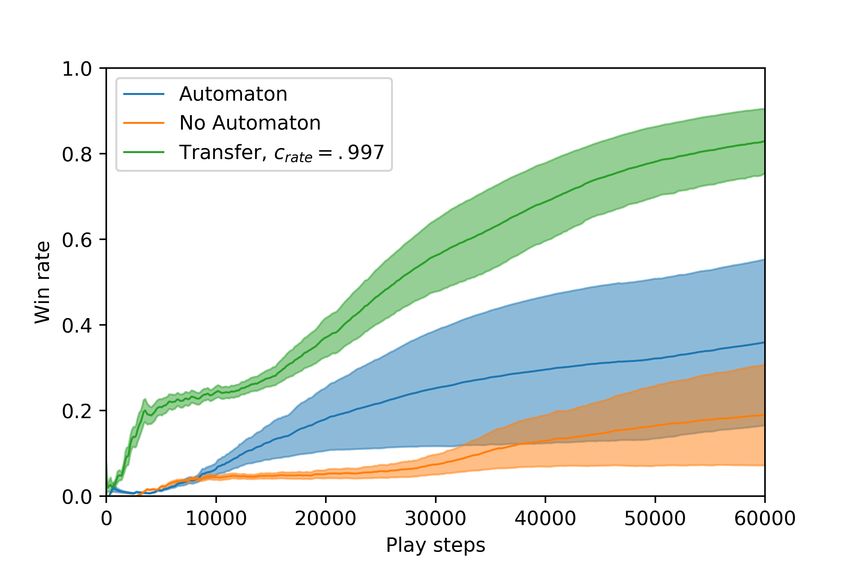
Figure 6: The performance of MCTSA with transfer learning episode number, tep , as seen in equation (6). This transfer
versus MCTSA without transfer learning and vanilla MCTS process allows for simple generalizations about an environ-
(No Automaton) as a function of play steps executed in the ment’s relationship with the objective structure to be learned
25 × 25 blind craftsman environment. Average win rate and on a smaller scale first. The automaton statistics learned
variance are reported for 25 randomly generated instances from the 10 × 10 grid guide the early learning process for
of the environment. all 25 × 25 environment runs.
The benefits of the automaton-guided transfer learning is
evident in the Blind Craftsman and Treasure Pit environ-
ments, as demonstrated in Figures 6 and 7.
VA (·) = ηtep VA10×10 (·)+(1−ηtep )VA25×25 (·), ηtep = (crate )tep
(6)
We train the 25×25 environment for 60k play steps, using
the same hyperparameters and network architecture as our
10 × 10 environments. This training process is repeated 25
times and the average win rates and variances of (i) utilizing
MCTSA with transfer learning, (ii) utilizing MCTSA with-
out transfer learning, and (iii) utilizing vanilla MCTS are re-
ported in Figures 6 and 7. In both of these instances, we ob-
serve the agent leveraging the transferred automaton statis-
tics has a higher and steeper win rate curve than MCTSA ,
and MCTSA performs better on average than vanilla MCTS.
Figure 7: The win rate and variance are reported for MCTSA We hypothesize that automaton-guided transfer learning has
with transfer learning, MCTSA without transfer learning, the most advantage when facilitating the scheduling of sub-
and vanilla MCTS (No Automaton) as a function of the num- goals over complex board structures. We train the 25x25 en-
ber of play steps executed in 25 instances of 25×25 Treasure vironment with the same hyper-parameters and network ar-
Pit environments. chitecture as in the previous section.
Transfer Learning
We also investigated using the automaton transition values Conclusion
VA of the objective automaton as a transfer learning mecha-
nism between different environment instances that share the MCTSA is proposed as a means to integrate novel reward
same objective. A more complex version of the Blind Crafts- shaping functions based on automaton representations of
man and Treasure Pit environments is generated by scaling the underlying objective within modern implementations of
the grid size to 25 × 25. Given a 25 × 25 instance of an Monte Carlo Tree Search. In doing so, MCTSA simultane-
environment, we attempt to transfer learned transition val- ously reasons about both the state representation of the en-
ues from a simpler 10 × 10 version of the environment. The vironment and the automaton representation of the objec-
automaton-guided transfer learning procedure works as fol- tive. We demonstrate the effectiveness of our approach on
lows. First, the automaton transition values VA10×10 of the structured grid-world environments, such as those of Blind
objective automaton A are computed (Line 19 in Algorithm Craftsman and Treasure Pit. The automaton transition val-
2) for many randomly generated episodes of the 10 × 10 ues computed using MCTSA are shown to be a useful trans-
environment corresponding to a total of 500K play steps. fer learning mechanism between environments that share the
The exposure to these random grid layouts for a given envi- same objective but differ in size and layout.
12021Acknowledgements model-free reinforcement learning. In International Con-
This project is supported in part by the US Army/DURIP ference on Tools and Algorithms for the Construction and
program W911NF-17-1-0208 and NSF CAREER Award Analysis of Systems, 395–412. Springer.
CCF-1552497. Hasanbeig, M.; Abate, A.; and Kroening, D. 2018.
Logically-constrained reinforcement learning. arXiv
References preprint arXiv:1801.08099 .
Anthony, T.; Tian, Z.; and Barber, D. 2017. Thinking fast Hasanbeig, M.; Abate, A.; and Kroening, D. 2019. Certified
and slow with deep learning and tree search. In Advances in reinforcement learning with logic guidance. arXiv preprint
Neural Information Processing Systems, 5360–5370. arXiv:1902.00778 .
Brunello, A.; Montanari, A.; and Reynolds, M. 2019. Syn- Icarte, R. T.; Klassen, T.; Valenzano, R.; and McIlraith, S.
thesis of LTL formulas from natural language texts: State of 2018. Using reward machines for high-level task specifica-
the art and research directions. In 26th International Sym- tion and decomposition in reinforcement learning. In Inter-
posium on Temporal Representation and Reasoning (TIME national Conference on Machine Learning, 2107–2116.
2019). Schloss Dagstuhl-Leibniz-Zentrum fuer Informatik. Narvekar, S.; Peng, B.; Leonetti, M.; Sinapov, J.; Taylor,
Camacho, A.; Baier, J. A.; Muise, C.; and McIlraith, S. A. M. E.; and Stone, P. 2020. Curriculum learning for rein-
2018a. Finite LTL synthesis as planning. In Twenty- forcement learning domains: A framework and survey. Jour-
Eighth International Conference on Automated Planning nal of Machine Learning Research 21(181): 1–50.
and Scheduling. Ng, A. Y.; Harada, D.; and Russell, S. 1999. Policy invari-
Camacho, A.; Chen, O.; Sanner, S.; and McIlraith, S. A. ance under reward transformations: Theory and application
2017. Non-Markovian rewards expressed in LTL: guiding to reward shaping. In ICML, volume 99, 278–287.
search via reward shaping. In Tenth Annual Symposium on Sadigh, D.; Kim, E. S.; Coogan, S.; Sastry, S. S.; and Seshia,
Combinatorial Search. S. A. 2014. A learning based approach to control synthe-
Camacho, A.; Chen, O.; Sanner, S.; and McIlraith, S. A. sis of Markov decision processes for linear temporal logic
2018b. Non-Markovian rewards expressed in LTL: Guiding specifications. In 53rd IEEE Conference on Decision and
search via reward shaping (extended version). In GoalsRL, Control, 1091–1096. IEEE.
a workshop collocated with ICML/IJCAI/AAMAS. Schrittwieser, J.; Antonoglou, I.; Hubert, T.; Simonyan, K.;
Camacho, A.; Icarte, R. T.; Klassen, T. Q.; Valenzano, R. A.; Sifre, L.; Schmitt, S.; Guez, A.; Lockhart, E.; Hassabis, D.;
and McIlraith, S. A. 2019. LTL and Beyond: Formal Lan- Graepel, T.; et al. 2020. Mastering atari, go, chess and shogi
guages for Reward Function Specification in Reinforcement by planning with a learned model. Nature 588(7839): 604–
Learning. In IJCAI, volume 19, 6065–6073. 609.
Chen, Y.; Chen, Y.; Yang, Y.; Li, Y.; Yin, J.; and Fan, C. Silver, D.; Huang, A.; Maddison, C. J.; Guez, A.; Sifre, L.;
2019. Learning action-transferable policy with action em- Van Den Driessche, G.; Schrittwieser, J.; Antonoglou, I.;
bedding. arXiv preprint arXiv:1909.02291 . Panneershelvam, V.; Lanctot, M.; et al. 2016. Mastering the
game of Go with deep neural networks and tree search. na-
De Giacomo, G.; De Masellis, R.; and Montali, M. 2014. ture 529(7587): 484.
Reasoning on LTL on finite traces: Insensitivity to infinite-
ness. In Twenty-Eighth AAAI Conference on Artificial Intel- Silver, D.; Hubert, T.; Schrittwieser, J.; Antonoglou, I.; Lai,
ligence. M.; Guez, A.; Lanctot, M.; Sifre, L.; Kumaran, D.; Graepel,
T.; et al. 2018. A general reinforcement learning algorithm
De Giacomo, G.; and Vardi, M. 2015. Synthesis for LTL and that masters chess, shogi, and Go through self-play. Science
LDL on finite traces. In Twenty-Fourth International Joint 362(6419): 1140–1144.
Conference on Artificial Intelligence.
Silver, D.; Schrittwieser, J.; Simonyan, K.; Antonoglou, I.;
Devlin, J.; Chang, M.-W.; Lee, K.; and Toutanova, K. 2018. Huang, A.; Guez, A.; Hubert, T.; Baker, L.; Lai, M.; Bolton,
Bert: Pre-training of deep bidirectional transformers for lan- A.; et al. 2017. Mastering the game of Go without human
guage understanding. arXiv preprint arXiv:1810.04805 . knowledge. Nature 550(7676): 354.
Enzenberger, M.; Müller, M.; Arneson, B.; and Segal, Taylor, M. E.; and Stone, P. 2009. Transfer learning for rein-
R. 2010. Fuego—an open-source framework for board forcement learning domains: A survey. Journal of Machine
games and Go engine based on Monte Carlo tree search. Learning Research 10(Jul): 1633–1685.
IEEE Transactions on Computational Intelligence and AI in Toro Icarte, R.; Klassen, T. Q.; Valenzano, R.; and McIlraith,
Games 2(4): 259–270. S. A. 2018. Teaching multiple tasks to an RL agent using
Gaon, M.; and Brafman, R. 2020. Reinforcement Learning LTL. In Proceedings of the 17th International Conference
with Non-Markovian Rewards. In Proceedings of the AAAI on Autonomous Agents and MultiAgent Systems, 452–461.
Conference on Artificial Intelligence, volume 34, 3980– International Foundation for Autonomous Agents and Mul-
3987. tiagent Systems.
Hahn, E. M.; Perez, M.; Schewe, S.; Somenzi, F.; Trivedi, Toro Icarte, R.; Waldie, E.; Klassen, T.; Valenzano, R.; Cas-
A.; and Wojtczak, D. 2019. Omega-regular objectives in tro, M.; and McIlraith, S. 2019. Learning reward machines
12022for partially observable reinforcement learning. Advances in
Neural Information Processing Systems 32: 15523–15534.
Weiss, K.; Khoshgoftaar, T. M.; and Wang, D. 2016. A sur-
vey of transfer learning. Journal of Big data 3(1): 1–40.
Xu, Z.; Gavran, I.; Ahmad, Y.; Majumdar, R.; Neider, D.;
Topcu, U.; and Wu, B. 2020. Joint inference of reward ma-
chines and policies for reinforcement learning. In Proceed-
ings of the International Conference on Automated Planning
and Scheduling, volume 30, 590–598.
12023You can also read