Earth system data cubes unravel global multivariate dynamics - Earth System Dynamics
←
→
Page content transcription
If your browser does not render page correctly, please read the page content below
Earth Syst. Dynam., 11, 201–234, 2020
https://doi.org/10.5194/esd-11-201-2020
© Author(s) 2020. This work is distributed under
the Creative Commons Attribution 4.0 License.

                              Earth system data cubes unravel
                                global multivariate dynamics
       Miguel D. Mahecha1,2,3, , Fabian Gans1, , Gunnar Brandt4 , Rune Christiansen5 , Sarah E. Cornell6 ,
       Normann Fomferra4 , Guido Kraemer1,2,7 , Jonas Peters5 , Paul Bodesheim1,8 , Gustau Camps-Valls7 ,
       Jonathan F. Donges6,9 , Wouter Dorigo10 , Lina M. Estupinan-Suarez1,12 , Victor H. Gutierrez-Velez11 ,
      Martin Gutwin1,12 , Martin Jung1 , Maria C. Londoño13 , Diego G. Miralles14 , Phillip Papastefanou15 , and
                                              Markus Reichstein1,2,3
                                 1 Max     Planck Institute for Biogeochemistry, Jena, Germany
            2 German   Centre for Integrative Biodiversity Research (iDiv), Deutscher Platz 5e, Leipzig, Germany
                     3 Michael Stifel Center Jena for Data-Driven and Simulation Science, Jena, Germany
                                         4 Brockmann Consult GmbH, Hamburg, Germany
                 5 Department of Mathematical Sciences, University of Copenhagen, Copenhagen, Denmark
                           6 Stockholm Resilience Center, Stockholm University, Stockholm, Sweden
                                 7 Image Processing Lab, Universitat de València, Paterna, Spain
                          8 Computer Vision Group, Friedrich Schiller University Jena, Jena, Germany
             9 Earth System Analysis, Potsdam Institute for Climate Impact Research, PIK, Potsdam, Germany
                           10 Department of Geodesy and Geo-Information, TU Wien, Vienna, Austria
                 11 Department of Geography and Urban Studies, Temple University, Philadelphia, PA, USA
                        12 Department of Geography, Friedrich Schiller University Jena, Jena, Germany
                   13 Alexander von Humboldt Biological Resources Research Institute, Bogotá, Colombia
                                    14 Hydro-Climate Extremes Lab (H-CEL), Ghent, Belgium
           15 TUM School of Life Sciences Weihenstephan, Technical University of Munich, Freising, Germany
                                          These authors contributed equally to this work.

                        Correspondence: Miguel D. Mahecha (miguel.mahecha@uni-leipzig.de)
                                         and Fabian Gans (fgans@bgc-jena.mpg.de)

                                   Received: 8 October 2019 – Discussion started: 9 October 2019
                       Revised: 7 February 2020 – Accepted: 17 February 2020 – Published: 25 February 2020

      Abstract. Understanding Earth system dynamics in light of ongoing human intervention and dependency re-
      mains a major scientific challenge. The unprecedented availability of data streams describing different facets
      of the Earth now offers fundamentally new avenues to address this quest. However, several practical hurdles,
      especially the lack of data interoperability, limit the joint potential of these data streams. Today, many initia-
      tives within and beyond the Earth system sciences are exploring new approaches to overcome these hurdles and
      meet the growing interdisciplinary need for data-intensive research; using data cubes is one promising avenue.
      Here, we introduce the concept of Earth system data cubes and how to operate on them in a formal way. The
      idea is that treating multiple data dimensions, such as spatial, temporal, variable, frequency, and other grids
      alike, allows effective application of user-defined functions to co-interpret Earth observations and/or model–
      data integration. An implementation of this concept combines analysis-ready data cubes with a suitable analytic
      interface. In three case studies, we demonstrate how the concept and its implementation facilitate the execu-
      tion of complex workflows for research across multiple variables, and spatial and temporal scales: (1) summary
      statistics for ecosystem and climate dynamics; (2) intrinsic dimensionality analysis on multiple timescales; and
      (3) model–data integration. We discuss the emerging perspectives for investigating global interacting and cou-
      pled phenomena in observed or simulated data. In particular, we see many emerging perspectives of this approach

Published by Copernicus Publications on behalf of the European Geosciences Union.
202                                                                 M. D. Mahecha et al.: The Earth System Data Lab concept

       for interpreting large-scale model ensembles. The latest developments in machine learning, causal inference, and
       model–data integration can be seamlessly implemented in the proposed framework, supporting rapid progress in
       data-intensive research across disciplinary boundaries.

1   Introduction                                                    discoverability, (ii) access barriers, e.g. restrictive data use
                                                                    policies, (iii) lack of capacity building for interpretation, e.g.
Predicting the Earth system’s future trajectory given ongoing       understanding the assumptions and suitable areas of applica-
human intervention into the climate system and land surface         tion, (iv) quality and uncertainty information, (v) persistency
transformations requires a deep understanding of its func-          of data sets and evolution of maintained data sets, (vi) repro-
tioning (Schellnhuber, 1999; IPCC, 2013). In particular, it         ducibility for independent researchers, (vii) inconsistencies
requires unravelling the complex interactions between the           in naming or unit conventions, and (viii) co-interpretability,
Earth’s subsystems, often termed as “spheres”: atmosphere,          e.g. either due to spatiotemporal alignment issues or physi-
biosphere, hydrosphere (including oceans and cryosphere),           cal inconsistencies, among others. Some of these issues are
pedosphere, or lithosphere, and increasingly the “anthropo-         relevant to specific data streams and scientific communities
sphere”. The grand opportunity today is that many key pro-          only. In most cases, however, these issues reflect the neglect
cesses in various subsystems of the Earth are constantly mon-       of the FAIR principles (to be “findable, accessible, interop-
itored. Networks of ecological, hydrometeorological, and at-        erable, and re-usable”; Wilkinson et al., 2016). If the lack
mospheric in situ measurements, for instance, provide con-          of FAIR principles and limited (co-)interpretability come to-
tinuous insights into the dynamics of the terrestrial water and     gether, they constitute a major obstacle in science and slow
carbon fluxes (Dorigo et al., 2011; Baldocchi, 2014; Wingate        down the path to new discoveries. Or, to put it as a challenge,
et al., 2015; Mahecha et al., 2017). Earth observations re-         we need new solutions that minimize the obstacles that hin-
trieved from satellite remote sensing enable a synoptic view        der scientists from capitalizing on the existing data streams
of the planet and describe a wide range of phenomena in             and accelerate scientific progress. More specifically, we need
space and time (Pfeifer et al., 2012; Skidmore et al., 2015;        interfaces that allow for interacting with a wide range of data
Mathieu et al., 2017). The subsequent integration of in situ        streams and enable their joint analysis either locally or in the
and space-derived data, e.g. via machine learning methods,          cloud.
leads to a range of unprecedented quasi-observational data             As long as we do not overcome data interoperability
streams (e.g. Tramontana et al., 2016; Balsamo et al., 2018;        limitations, Earth system sciences cannot fully exploit the
Bodesheim et al., 2018; Jung et al., 2019). Likewise, diagnos-      promises of novel data-driven exploration and modelling ap-
tic models that encode basic process knowledge, but which           proaches to answer key questions related to rapid changes in
are essentially driven by observations, produce highly rele-        the Earth system (Karpatne et al., 2018; Bergen et al., 2019;
vant data products (see, e.g. Duveiller and Cescatti, 2016;         Camps-Valls et al., 2019; Reichstein et al., 2019). A variety
Jiang and Ryu, 2016a; Martens et al., 2017; Ryu et al., 2018).      of approaches have been developed to interpret Earth obser-
Many of these derived data streams are essential for monitor-       vations and big data in the Earth system sciences in general
ing the climate system including land surface dynamics (see,        (for an overview, see, e.g. Sudmanns et al., 2019) and gridded
for instance, the essential climate variables, ECVs; Hollmann       spatiotemporal data as a special case (Nativi et al., 2017; Lu
et al., 2013; Bojinski et al., 2014), oceans at different depths    et al., 2018). For the latter, data cubes have recently become
(essential ocean variables, EOVs; Miloslavich et al., 2018),        popular, addressing an increasing demand for efficient ac-
or the various aspects of biodiversity (essential biodiversity      cess, analysis, and processing capabilities for high-resolution
variables, EBVs; Pereira et al., 2013). Together, these essen-      remote sensing products. The existing data cube initiatives
tial variables describe the state of the planet at a given mo-      and concepts (e.g. Baumann et al., 2016; Lewis et al., 2017;
ment in time and are indispensable for evaluating Earth sys-        Nativi et al., 2017; Appel and Pebesma, 2019; Giuliani et al.,
tem models (Eyring et al., 2019).                                   2019) vary in their motivations and functionalities. Most of
   With regard to the acquisition of sensor measurements and        the data cube initiatives are, however, motivated by the need
the derivation of downstream data products, Earth system            for accessing singular (very-)high-resolution data cubes, e.g.
sciences are well prepared. But can this multitude of data          from satellite remote sensing or climate reanalysis, and not
streams be used efficiently to diagnose the state of the Earth      by the need for global multivariate data exploitation.
system? In principle, our answer would be affirmative, but             This paper has two objectives: first, we aim to formalize
in practical terms we perceive high barriers to interconnect-       the idea of an Earth system data cube (ESDC) that is tai-
ing multiple data streams and further linking these to data         lored to explore a variety of Earth system data streams to-
analytic frameworks (as discussed for the EBVs by Hardisty          gether and thus largely complements the existing approaches.
et al., 2019). Examples of these issues are (i) insufficient data   The proposed mathematical formalism intends to illustrate

Earth Syst. Dynam., 11, 201–234, 2020                                                  www.earth-syst-dynam.net/11/201/2020/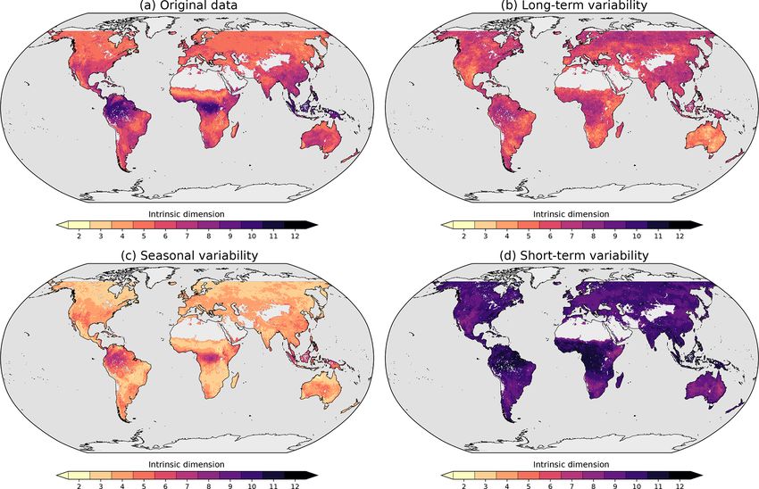
M. D. Mahecha et al.: The Earth System Data Lab concept                                                                           203

how one can efficiently operate such data cubes. Second,                then identified as different coordinates in the multivariate
the paper aims at introducing the Earth System Data Lab                 array Y . However, when calculating simple variable sum-
(ESDL; https://earthsystemdatalab.net, last access: 21 Febru-           maries or performing spatiotemporal aggregations of the
ary 2020). The ESDL is an integrated data and analytical                data, such a representation can be computationally obstruc-
hub that curates a multitude of data streams representing key           tive. We therefore propose to consider the “variable indica-
processes of the different subsystems of the Earth in a com-            tor” k ∈ {1, . . . , p} as simply another dimension of the in-
mon data model and coordinate reference system. This in-                dex set and view the data as the collection {Xi }i∈I of uni-
frastructure enables researchers to apply their user-defined            variate observations, where I = J × {1, . . . , p}1 and where
functions (UDFs) to these analysis-ready data (ARD). To-                X(j,k) := Yjk . With this idea in mind, we now formally define
gether, these elements minimize the hurdle to co-explore a              the Earth system data cube (“data cube” in short).
multitude of Earth system data streams. Most known initia-                 A data cube C consists of a triplet (L, G, X) of compo-
tives intend to preserve the resolutions of the underlying data         nents to be described below.
and facilitate their direct exploitation, like the Earth Server
(Baumann et al., 2016) or the Google Earth Engine (Gore-                  – L is a set of labels, called dimensions, describing the
lick et al., 2017). The ESDL, instead, is built around singular             axes of the data cube. For example, L = {lat, long, time,
data cubes on common spatiotemporal grids that include a                    var} describes a data cube containing spatiotemporal
high number of variables as a dimension in its own right.                   observations from a range of different variables. The
This design principle is thought to be advantageous com-                    number of dimensions |L| is referred to as the order of
pared to building data cubes from individual data streams                   cube C; in the above example, |L| = 4.
without considering their interactions from the very begin-               – G is a collection {grid(`)}`∈L of grids along the axes
ning. Due to its multivariate structure and the easy-to-use in-             in L. For every ` ∈ L, the set grid(`) is a discrete sub-
terface, the ESDL is well suited for being part of data-driven              set of the domain of the axis `, specifying the resolu-
challenges, as regularly organized by the machine learning                  tion at which data are available along this axis. Every
community, for example.                                                     set grid(`) is required to contain at least two elements.
   The remainder of the paper is organized as follows: Sect. 2              Dimensions containing only one grid point are dropped.
introduces the concept based on a formal definition of Earth                The collection G defines the hyper-rectangular index set
system data cubes and explains how user-defined functions
can interact with them. In Sect. 3, we describe the imple-                   I (G) :=     grid(`), motivating the name “cube”. For ex-
mentation of the Earth System Data Lab in the programming                    ample,
language Julia and as a cloud-based data hub. Section 4 then
illustrates three research use cases that highlight different                I (G) =      grid(`)
ways to make use of the ESDL. We present an example from                           = grid(lat) × grid(long) × grid(time) × grid(var)
an univariate analysis, characterizing seasonal dynamics of                       = {−89.75, . . ., 89.75} × {−179.75, . . ., 179.75}
some selected variables; an example from high-dimensional
                                                                                  ×{1 Jan 2010, . . ., 31 Dec 2010} × GPP, SWC, Rg
data analysis; and an example for the representation of a
model–data integration approach. In Sect. 5, we discuss the                       = {(−89.75, −179.75, 1 Jan 2010, GPP),

current advantages and limitations of our approach and put                        . . ., 89.75, 179.75, 31 Dec 2010, Rg .
an emphasis on required future developments.
                                                                             Since G and I (G) are in one-to-one correspondence, we
                                                                             will use the two interchangeably.
2   Concept
                                                                          – X is a collection of data {Xi }i∈I (G) ⊆ RNA := R ∪ {NA}
                                                                            observed at the grid points in I (G). Here, “NA” refers
Our vision is that multiple spatiotemporal data streams shall
                                                                            to “not available”.
be treated as a singular yet potentially very high-dimensional
data stream. We call this singular data stream an Earth system             In this view, the data can be treated as a collection
data cube. For the sake of clarity, we introduce a mathemat-            {Xi }i∈I (G) of univariate observations, even if they encode
ical representation of the Earth system data cube and define            different variables. In the above example, the variable axis is
operations on it. Further details on an efficient implementa-           a nominal grid with the entries GPP (gross primary produc-
tion are provided in Sect. 3.2 and 3.3.                                 tion), SWC (soil water content), and Rg (global radiation).
   Suppose we observe p variables Y 1 , . . ., Y p , each under         The set of all data cubes with dimensions L will be denoted
a (possibly different) range of conditions. A first step to-            by C(L). Data cubes that contain one variable only can be
wards data integration is to (re)sample all data streams onto           considered as special case; other common choices of L are
a common domain J (e.g. a spatiotemporal grid) to ob-                   described in Table 1. The list of example axes labels used in
                                      p
tain the indexed set {(Yj1 , . . . , Yj )}j ∈J of multivariate obser-
vations. Observations obtained from different variables are                1 The symbol     indicates a Cartesian product.

www.earth-syst-dynam.net/11/201/2020/                                                        Earth Syst. Dynam., 11, 201–234, 2020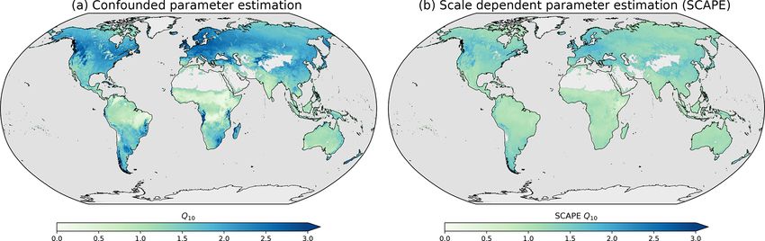
204                                                                 M. D. Mahecha et al.: The Earth System Data Lab concept

the table is, of course, not exhaustive. Other relevant dimen-      A∩R = ∅ by executing the described “apply” operation. The
sions could be, for example, model versions, model parame-          code package accompanying this paper (described in Sect. 3)
ters, quality flags, or uncertainty estimates. Note that, by def-   automatically equips every UDF with such a functionality. A
inition, a data cube only depends on its dimensions through         schematic description of this approach is illustrated in Fig. 1.
the set of axes L and is therefore indifferent to any order            The approach outlined above is very convenient to
of these. In the remainder of this article, the notion of data      describe workflows, i.e. recursive chains of UDFs. Let
cubes refers to this concept. Note that dropping dimensions         f1 , . . . fn be a sequence of UDFs with corresponding min-
that only contain one grid point is not the only possible way       imal input/output dimensions (E1 , R1 ), . . . , (En , Rn ). If an
of working with data cubes. Another equally valid idea is to        output dimension Ri is a subset of subsequent input Ei+1 ,
maintain grids of length 1 and integrate them to the workflow.      we can chain these functions. A recursive workflow emerges
                                                                    when Ri ⊆ Ei+1 for all i, by iteratively chaining f1 , . . . , fn
2.1   Operations on an Earth system data cube                       upon one another. The input/output dimensions of the result-
                                                                    ing cube are (E1 , Rn ).
To exploit an Earth system data cube efficiently, scientific           Overall, the definition of an Earth system data cube and
workflows need to be translated into operations executable          associated operations on it do not only guide the imple-
on data cubes as described above. More specifically, the out-       mentation strategy but also help us summarize potentially
put of each operation on a data cube should yield another data      complicated analytic procedures in a common language. For
cube. The entire workflow of a project, possibly a succession       the sake of readability, in the following, we will not distin-
of analyses performed by different collaborators, can then          guish between a function f (defined only for minimal input)
be expressed as a composition of several UDFs performed             and its extension f (equipped with the apply functionality;
on a single (input) data cube. Besides unifying all statistical     see Fig. 1). The former will be referred to as an “atomic”
data analyses into a common concept, the idea of express-           function. We typically indicate the minimal input/output di-
ing workflows as functional operations on data cubes comes          mensions (E, R) of a function f by writing fER . Since the
with another important advantage: as soon as a workflow is          pair (E, R) does not determine the mapping f , this notation
implemented as a suitable set of UDFs, it can be reused on          should not be understood as the parameterization of a func-
any other sufficiently similar data cube to produce the same        tion class but rather provide an easy way to perform input
kind of output.                                                     control and to anticipate the output dimensions of a cube re-
   In its most general form, a user-defined function C 7 −→         turned by f . For instance, following the discussion above, a
f (C) operates by (i) extracting relevant information from C,       function denoted by fER can be applied to any cube with di-
(ii) performing calculations on the extracted information, and      mension E ∪A, satisfying that A∩R = ∅, and returns a cube
(iii) storing these calculations into a new data cube f (C). In     with dimensions R ∪ A. To avoid ambiguities, additional no-
order to perform step (i), f expects a minimal set of dimen-        tation is needed when distinguishing between two functions
sions E of the input cube. The returned set of axes for an          with the same pair of minimal input/output dimensions.
input cube with dimensions E will be denoted by R. That is,
f is a mapping such that
                                                                    2.2    Examples
f : C(E) → C(R).                                             (1)    In the following, we present some special operations that are
Alongside the function f , one has to define the sets E and R,      routinely needed in explorations of Earth system data cubes:
which we will refer to as minimal input and minimal output             “Reducing” describes a function that calculates some
dimensions, respectively.                                           scalar measure (e.g. the sample mean). Consider, for in-
   A major advantage of thinking in data cube workflows             stance, the need to estimate the mean of a univariate data
is that low-dimensional functions can be applied to higher-         cube, of course weighted by the area of the spatial grid cells.
dimensional cubes by simple functional extensions: a func-          An operation of this kind expects a cube with dimensions
tion can be acting along a particular set of dimensions while       E = {lat, long, time} and returns a cube with dimensions
looping across all unspecified dimensions. For example, the         R = { } and is therefore a mapping:
function that computes the temporal mean of a univariate              {}
                                                                    f{lat,long,time} : C({lat, long, time}) → C({ }).             (2)
time series should allow for an input data cube, which, in
addition to a temporal grid, contains spatial information. The      This mapping can now be applied to any data cube of po-
output of such an operation should then be a cube of spa-           tentially higher (but not lower) dimensionality. For instance,
tially gridded temporal means. Similarly, the function should       f is automatically extended to a multivariate spatiotemporal
be applicable to cubes containing multivariate observations.        data cube (Table 1) with the mapping
Here, we expect the output to contain one temporal mean per
supplied variable.                                                    {}
                                                                    f{lat,long,time} : C({lat, long, time, var}) → C({var}),      (3)
   In general, a function f defined on C(E) should natu-
rally extend to a function from C(E ∪ A) to C(R ∪ A) with           which computes one spatiotemporal mean for each variable.

Earth Syst. Dynam., 11, 201–234, 2020                                                   www.earth-syst-dynam.net/11/201/2020/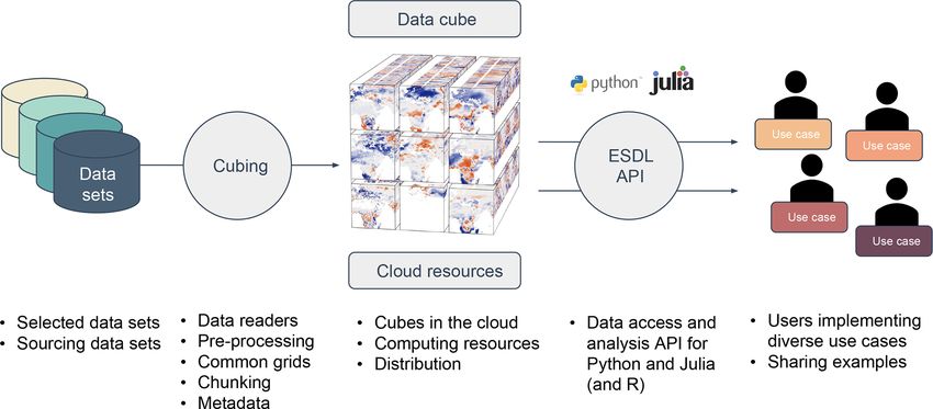
M. D. Mahecha et al.: The Earth System Data Lab concept                                                                                   205

Table 1. Typical sets of data cubes C(L) of varying orders |L| with characteristic dimensions L.

                 Order |L|    Set of data cubes C(L)           Description of C(L)
                 0            C({})                            Scalar value where no dimension is defined
                 1            C({lat})                         Univariate latitudinal profile
                 1            C({long})                        Univariate longitudinal profile
                 1            C({time})                        Univariate time series
                 1            C({var})                         Single multivariate observation
                 2            C({lat, long})                   Univariate static geographical map
                 2            C({lat, time})                   Univariate Hovmöller diagram: zonal pattern over time
                 2            C({lat, var})                    Multivariate latitudinal profile
                 2            C({long, time})                  Univariate Hovmöller diagram: meridional pattern over time
                 2            C({long, var})                   Multivariate longitudinal profile
                 2            C({time, var})                   Multivariate time series
                 2            C({time, freq})                  Univariate time–frequency plane
                 3            C({lat, long, time})             Univariate data cube
                 3            C({lat, long, var})              Multivariate map, e.g. a global map of different soil properties
                 3            C({lat, time, var})              Multivariate latitudinal Hovmöller diagram
                 3            C({long, time, var})             Multivariate longitudinal Hovmöller diagram
                 3            C({time, freq, var})             Multivariate spectrally decomposed time series
                 4            C({lat, long, time, var})        Multivariate spatiotemporal cube
                 4            C({lat, long, time, freq})       Univariate spectrally decomposed data cube
                 5            C({lat, long, time, var, ens})   Multivariate ensemble of model simulations

Figure 1. Schematic illustration of the “apply” functionality: a function f : C(E) → C(R) is extended to the set of cubes with dimensions
E ∪ A, where A is an arbitrary set of dimensions with A ∩ R = ∅. Given a cube C ∈ C(E ∪ A), the extension f (C) is constructed by iterating
over all grid points i along the dimensions in A to obtain the collection {Ci } ⊆ C(E) of sliced cubes, applying f to every cube Ci separately,
and binding the collection {f (Ci )} into the output cube f (C) ∈ C(R ∪ A). Here, the index i runs through all elements in    grid(a).

www.earth-syst-dynam.net/11/201/2020/                                                           Earth Syst. Dynam., 11, 201–234, 2020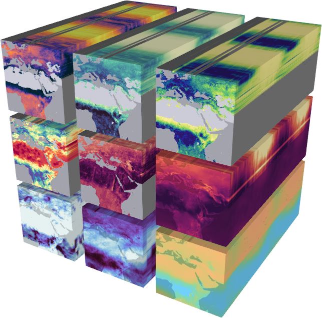
206                                                                         M. D. Mahecha et al.: The Earth System Data Lab concept

   “Cropping” is subsetting a data cube while maintaining                   3     Data streams and implementation
the order of a cube. A cropping operation typically reduces
certain axes of a data cube to only contain specified grid                  The concept as described in Sect. 2 is generic, i.e. inde-
points (and therefore requires the input cube to contain these              pendent of the implemented Earth system data cube and of
grid points). For instance, a function that extracts a certain              the technical solution of the implementation. Figure 2 shows
“cropped” fraction T0 along the temporal cover expects an                   how the concept outlined above is realized from a practical
input cube containing a time axis with a grid at least as highly            point of view. The flowchart shows that the starting point is
resolved as T0 . This function preserves the dimensionality of              the collection of relevant data streams which then need to
the cube but reduces the grid along the time axis; i.e.                     be preprocessed in order to be interpretable as a single data
 {time}                                                                     cube. The ESDC itself may be stored locally or in the cloud
f{time} : C ({time}|grid(time) ⊇ T0 ) → C ({time}|grid(time) = T0 ) , (4)
                                                                            and can be accessed from various users simultaneously based
where we have used C(L|P ) to denote the set of cubes with                  on different application programming interfaces (APIs). In
dimensions L satisfying the condition P . Thanks to the apply               the following, we firstly present the data used in our imple-
functionality, this atomic function can be used on any cube                 mentation of the ESDL which is available online, and sec-
of higher order. For example, it is readily extended to a map-              ondly describe the implementation strategy for the API we
ping:                                                                       developed in this project.
  {time}
f{time} :C ({lat, long, time}|grid(time) ⊇ T0 )
                                                                            3.1    Data streams in the ESDL
           → C ({lat, long, time}|grid(time) = T0 ) ,                 (5)
which crops the time axis of cubes with dimensions {lat,                    The data streams included so far were chosen to enable re-
long, time}. Analogously, all dimensions can be subsetted as                search on the following topics (a complete list is provided in
long as the length of the dimension is larger than 1. The latter            Appendix A):
would be called slicing.
                                                                                – Ecosystem states at the global scale in terms of rele-
   “Slicing” refers to a subsetting operation in which a di-
                                                                                  vant biophysical variables. Examples are leaf area in-
mension of the cube is degenerated, and the order of the
                                                                                  dex (LAI), the fraction of photosynthetically active ra-
cube is reduced and can be interpreted as a special form
                                                                                  diation (fAPAR), and albedo (Disney et al., 2016; Pinty
of cropping. For instance, if we only select a singular time
                                                                                  et al., 2006; Blessing and Löw, 2017).
instance t0 , the time dimension effectively vanishes as we
do not longer need a vector-spaced dimension to represent
                                                                                – Biosphere–atmosphere interactions as encoded in land
its values. When applied to a spatiotemporal data cube, this
                                                                                  fluxes of CO2 , i.e. GPP, terrestrial ecosystem respira-
amounts to a mapping:
                                                                                  tion (Reco ), and the net ecosystem exchange (NEE) as
 {}
f{time} : C ({lat, long, time}|grid(time) 3 t0 ) → C ({lat, long}).   (6)         well as the latent heat (LE) and sensible heat (H ) en-
                                                                                  ergy fluxes. Here, we rely mostly on the FLUXCOM
   “Expansions” are operations where the order of the output
                                                                                  data suite (Tramontana et al., 2016; Jung et al., 2019).
cube is higher than the order of the corresponding input cube.
A discrete spectral decomposition of time series, for exam-
                                                                                – Terrestrial hydrology requires a wide range of variables.
ple, generates a new dimension with characteristic frequency
                                                                                  We mainly ingest data from the Global Land Evapora-
classes:
                                                                                  tion Amsterdam Model (GLEAM; Martens et al., 2017;
  {time,freq}
f{time}         : C({time}) → C({time, freq}).                        (7)         Miralles et al., 2011) which provide a series of relevant
   “Multiple cube handling” is often needed, for instance,                        surface hydrological properties such as surface (SM)
when fitting a regression model where response and predic-                        and root-zone soil moisture (SMroot ) but also poten-
tions are stored in different cubes. Also, we may be interested                   tial evaporation (Ep ) and evaporative stress (S) condi-
in outputting the fitted values and the residuals in two sepa-                    tions, among others. Ingesting entire products such as
rate cubes. This amounts to an atomic operation:                                  GLEAM ensures internal consistency.
  {para},{time}
f{time,var},{time} :C({time, var}) × C({time})                                  – State of the atmosphere is described using data gener-
                                                                                  ated by the Climate Change Initiative (CCI) by the Eu-
                     → C({para}) × C({time}),                         (8)
                                                                                  ropean Space Agency (ESA) in terms of aerosol opti-
which expects a multivariate data cube for the predictors                         cal depth at different wavelengths (AOD550 , AOD555 ,
C1 ∈ C({time, var}) and a univariate cube for the targets C2 ∈                    AOD659 , and AOD1610 ; Holzer-Popp et al., 2013), to-
C({time}). The output consists of a vector of fitted parame-                      tal ozone column (Van Roozendael et al., 2012; Lerot
ters C̃1 ∈ C({para}) and a residual time series C̃2 ∈ C({time})                   et al., 2014), as well as surface ozone (which is more rel-
to compute the model performance. This concept also allows                        evant to plants), and total column water vapour (TCWV;
the integration of more than two input and/or output cubes.                       Schröder et al., 2012; Schneider et al., 2013).

Earth Syst. Dynam., 11, 201–234, 2020                                                           www.earth-syst-dynam.net/11/201/2020/
M. D. Mahecha et al.: The Earth System Data Lab concept 207
Figure 2. Workflow putting the ESDL concept into practice: selected data sets are preprocessed to common grids and saved in cloud-ready
data formats (Zarr). Based on these cubed data sets, a global Earth system data cube can be produced that is either stored locally or in the
cloud. Via appropriate application programming interfaces (APIs), users can efficiently access the ESDC in their native language. Users can
fully focus on designing user-defined functions and workflows.
– Meteorological conditions are described via the reanal- rent applicability in biodiversity studies at regional scales.
ysis data, i.e. the ERA5 product. Additionally, precipita- Data layers from governmental organizations providing de-
tion is ingested from the Global Precipitation Climatol- tailed information about ecosystems are also available that
ogy Project (GPCP; Adler et al., 2003; Huffman et al., allow a national characterization and deeper understanding
2009). of ecosystem changes by natural or human drivers. These are
maps of biotic units (Londoño et al., 2017), wetlands (Flórez
Together, these data streams form data cubes of intermedi- et al., 2016), and agriculture frontier maps (MADR-UPRA,
ate spatial and temporal resolutions (0.25, 0.083◦ ; both 8 d), 2017). Additionally, GPP, evapotranspiration, shortwave ra-
visualized in Fig. 3. The variables described here are de- diation, PAR, and diffuse PAR from the Breathing Earth Sys-
scribed in more detail in a list provided in Appendix A, which tem Simulator (BESS; Ryu et al., 2011, 2018; Jiang and Ryu,
may, however, already be incomplete at the time of publica- 2016b) and albedo from QA4ECV (http://www.qa4ecv.eu/,
tion, as the ESDL is a living data suite, constantly expanding last access: 21 February 2020) are available, among others.
according to users’ requests. For the latest overview, we refer This regional Earth system data cube should serve as a plat-
the reader to the website (https://www.earthsystemdatalab. form for analysis in a region with variability of landscape,
net/, last access: 21 February 2020). Note that we have not high biodiversity and ecosystem transitions gradients, and
considered the integration of uncertainty as another dimen- facing rapid land use change (Sierra et al., 2017).
sion in the current implementation. The rationale is that each
of the data products comes with a specific uncertainty flag or
3.2 Implementation
estimate that cannot be merged in an own dimension. This is
an open aspect that needs to be addressed in future develop- To put the concept of an Earth system data cube as out-
ments. lined in Sect. 2 into practice, we need suitable access APIs
To show the portability of the approach, we have devel- (see Fig. 2). A co-author of this paper (FG) developed one
oped a regional data cube for Colombia. This work supports API in the relatively young scientific programming language
the Colombian Biodiversity Observational Network activities Julia (https://julialang.org/, last access: 21 February 2020;
within the Group on Earth Observations Biodiversity Obser- Bezanson et al., 2017) which is provided via the ESDL.jl
vation Network (GEO BON). This regional data cube has package. Additionally, all functionalities are also available
a 1 km (0.083◦ ) resolution and focuses on remote-sensing- in Python based on existing libraries and documented online.
derived data products (i.e. LAI, fAPAR, the normalized dif- In both cases, the goal was that the user does not have to
ference vegetation index (NDVI), the enhanced vegetation explicitly deal with the complexities of sequential data in-
index (EVI), LST, and burnt area). In addition to the global put/output handling and can concentrate on implementing the
ESDL, monthly mean products such as cloud cover (Wil- atomic functions and workflows, while the system takes care
son and Jetz, 2016) have been ingested given their recur- of necessary out of core and out-of-memory computations.
www.earth-syst-dynam.net/11/201/2020/ Earth Syst. Dynam., 11, 201–234, 2020208 M. D. Mahecha et al.: The Earth System Data Lab concept
Figure 3. Visualization of the implemented Earth system data cube (an animation is provided online at https://youtu.be/9L4-fq48Ev0, last
access: 21 February 2020). The figure shows from the top left to bottom right the variables sensible heat (H ), latent heat (LE), gross primary
production (GPP), surface moisture (SM), land surface temperature (LST), air temperature (Tair ), cloudiness (C), precipitation (P ), and water
vapour (V ). References to the individual data sources are given in Appendix A. Here, the resolution in space is 0.25◦ and 8 d in time, and we
are inspecting the time from May 2008 to May 2010; the spatial range is from 15◦ S to 60◦ N, and 10◦ E to 65◦ W.
The following is a sketched description of the principles of – Knowledge of the desired L and G allows us to develop
the Julia-based ESDL.jl implementation. We chose Julia to a suitable user-defined function fER .
translate the concepts outlined into efficient computer code
because it has clear advantages for data cube applications – Depending on the exact needs, mapslices and
besides its general elegance in scientific computing in terms mapCube will then be used to apply the fER on a cube
of speed, dynamic programming, multiple dispatch, and syn- as illustrated in Fig. 1. mapCube is a strict implementa-
tax (Perkel, 2019). Specifically, Julia allows for generic pro- tion of the cube mapping concept described here, where
cessing of high-dimensional data without large code repe- it is mandatory to explicitly describe E and R such that
titions. At the core of the Julia ESDL.jl toolbox are the the atomic function is fully operational. mapslices
mapslices and mapCube functions, which execute user- is a convenient wrapper around the mapCube func-
defined functions on the data cube as follows: tion that tries to impute the output dimensions given the
user function definition to ease the application of the
– Given some large data cube C = (L, G, X), the ESDL functions where the output dimensions are trivial. In-
function subsetcube(C) will retrieve a handle to C ternally, mapslices and mapCube verify that E ⊆ L
that fully describes L and G. and other conditions.
The case studies developed in Sect. 4 are accompanied by
code that illustrates this approach in practice.
Of course there are also alternatives to Julia. Lu et al.
(2018) recently reviewed different ways of applying func-
Earth Syst. Dynam., 11, 201–234, 2020 www.earth-syst-dynam.net/11/201/2020/M. D. Mahecha et al.: The Earth System Data Lab concept 209
tions on array data sets in R, Octave, Python, Rasdaman, and One disadvantage of the traditional file formats used for
SciDB. One requirement of such a mapping function is that it storing gridded data is that their data chunks are contained in
should be scalable, which means that it should process data single files that may become impossible to handle efficiently.
larger than the computer memory and, if needed, in paral- This is not problematic when the data are stored on a regular
lel. While existing solutions are sufficient for certain applica- file system where the file format library can read only parts
tions, most are not consistent with the cube mapping concept of the file. In cloud-based storage systems, it is not com-
as described in Sect. 2. For instance, the required handling of mon to have an API for accessing only parts of an object,
complex workflows of multiple cubes (Eq. 8) is typically not so these file formats are not well suited for being stored in
possible in the existing solutions that have been reviewed. In the cloud. Recently, novel solutions for this issue were pro-
some cases, issues in the computational efficiency of the un- posed, including modifications to existing storage formats,
derlying programming languages render certain solutions not e.g. HDF5 cloud, or cloud-optimized GeoTiff, among others,
suitable. This is particularly the case when user-defined func- as well as completely new storage formats, in particular Zarr
tions become complex. Likewise, certain properties such as (https://zarr.readthedocs.io/, last access: 21 February 2020)
the desired indifference to the ordering in axes dimensions and TileDB (https://tiledb.io/, last access: 21 February 2020).
are often not foreseen. One suitable alternative to Julia is While working with these formats is very similar to tradi-
available in Python. The xarray (http://xarray.pydata.org, tional solutions (like HDF5 and NetCDF), these new formats
last access: 21 February 2020) and dask packages have been are optimized for cloud storage as well as for parallel read
successfully utilized in the Open Data Cube, Pangeo, and and write operations. Here, we chose to use the new Zarr for-
xcube initiatives. Extensive descriptions on how to work in mat. The reason is that it enables us to share the data cube
the ESDL with both Python and Julia can be accessed from through an object storage service, where the data are public
the following website: https://www.earthsystemdatalab.net/ and can be analysed directly. Python packages for accessing
(last access: 21 February 2020). The open-source implemen- and analysing large N-dimensional data sets like xarray
tation of the ESDL also implies that one can easily extend the and dask, which make a wide range of existing tools read-
stored data sets. The online documentation shows in detail ily usable on the cube, and a Julia approach to read Zarr data
how additional data can be added to the ESDL. In particular, have been implemented as well.
if the data share common axes and are stored in a compatible At present, the ESDL provides the same data cube in dif-
format (as described below in Sect. 3.3), this does not require ferent spatial resolutions and different chunkings to speed up
major efforts. data access for different applications. In chunked data for-
mats, a large data set is split into smaller chunks, which can
3.3 Storage and processing of the data cube be seen as separate entities where each chunk is represented
by an object in an object store. There are several ways to
The ESDL has been built as a generic tool. It is prepared chunk a data cube. Consider the case of a multivariate spa-
to handle very large volumes of data. Storage techniques tiotemporal cube C({lat, long, time, var}). One common strat-
for large raster geodata are generally split into two cat- egy would be to treat every spatial map of each variable and
egories: database-like solutions like Rasdaman (Baumann time point as one chunk, which would result in a chunk size
et al., 1998) or SciDB (Stonebraker et al., 2013) access of |grid(lat)| × |grid(long)| × 1 × 1. However, because an ob-
data directly through file formats that follow metadata con- ject can only be accessed as a whole, the time for reading a
ventions like HDF5 (https://www.hdfgroup.org/, last ac- slice of a univariate data cube does not directly scale with
cess: 21 February 2020) or NetCDF (https://www.unidata. the number of data points accessed but rather with the num-
ucar.edu/software/netcdf/, last access: 21 February 2020). ber of accessed chunks. Reading out a univariate time se-
Database solutions shine in settings where multiple users re- ries of length 100 from this cube would require accessing
peatedly request (typically small) subsets of data cube, which 100 chunks. If one stored the same data cube with complete
might not be rectangular, because the database can acceler- time series contained in one chunk, read operations could
ate access by adjusting to common access patterns. However, perform much faster. Table 2 shows an overview of the im-
for batch processing large portions of a data cube, every data plemented chunkings for different cubes in the current ESDL
entry is ideally accessed only once during the whole compu- environment.
tation. Hence, when large fractions of some data cube have to
be accessed, users will usually avoid the overhead of build-
ing and maintaining a database and rather aim for accessing 4 Experimental case studies
the data directly from their files. This experience is often per-
ceived as more “natural” for Earth system scientists who are The overarching motivation for building an Earth system data
used to “touching” their data, knowing where files are lo- cube is to support the multifaceted needs of Earth system sci-
cated, and so forth. Databases instead offer, by construction, ences. Here, we briefly describe three case studies of vary-
an entry point to an otherwise unknown data set. ing complexity (estimating seasonal means per latitude, di-
mensionality reduction, and model–data integration) to illus-
www.earth-syst-dynam.net/11/201/2020/ Earth Syst. Dynam., 11, 201–234, 2020210 M. D. Mahecha et al.: The Earth System Data Lab concept
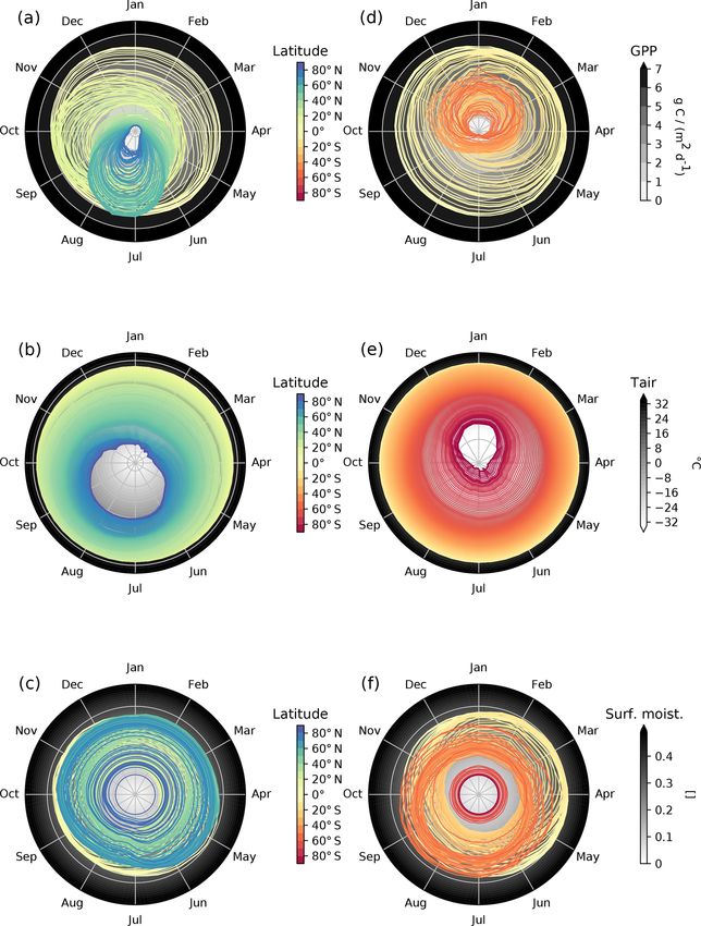
Table 2. Resolutions and chunkings of the currently implemented the background is the actual value of the variable. Together,
global Earth system data cube per variable. Here, the cubes with the left and right plots describe the global dynamics of phe-
chunk size 1 in the time coordinate are optimized for accessing nology, often referred to as the “green wave” (Schwartz,
global maps at a time, while the other cubes are more suited for 1998). We clearly see the almost nonexistent GPP in high-
processing time series or regional subsets of the data cube. The latitude winters and also find the imprint of constantly low to
cubes are currently hosted on the Object Storage Service by the
intermediate productivity values at latitudes that are charac-
Open Telecom Cloud under https://obs.eu-de.otc.t-systems.com/
obs-esdc-v2.0.0/ (last access: 21 February 2020) (state: Septem-
terized by dry ecosystems. Pronounced differences between
ber 2019). Northern and Southern Hemisphere reflect the very different
distribution of productive land surface.
Resolution Chunk size along axis For temperature, the observed seasonal dynamics are less
complex. We essentially find the constantly high temperature
Grid Grid Grid conditions near the Equator and visualize the pronounced
(time) (lat) (long)
seasonality at high latitudes. However, Fig. 4 also shows that
0.083◦ 184 270 270 temperature peaks lag behind the June/December solstices
0.083◦ 1 2160 4320 in the Northern Hemisphere, while in the Southern Hemi-
0.25◦ 184 90 90 sphere, the asymmetry of the seasonal cycle in temperature
0.25◦ 1 720 1440 is less pronounced. While the seasonal temperature gradient
is a continuum, surface moisture shows a much more com-
plex pattern across latitudes, as reflected in summer/winter
trate how the concept of the Earth system data cube can be depressions in certain midlatitudes. For instance, a clear drop
put into practice. Clearly, these examples emerge from our at, e.g. latitudes of approximately 60◦ N and even stronger
own research interest, but the concepts should be portable depressions in latitudinal bands dominated by dry ecosys-
across different branches of science (the code for producing tems.
the results on display is provided as Jupyter notebooks at This example analysis is intended to illustrate how the se-
https://github.com/esa-esdl/ESDLPaperCode.jl, last access: quential application of two basic functions on this Earth sys-
21 February 2020). tem data cube can unravel global dynamics across multiple
variables. We suspect that applications of this kind can lead
4.1 Inspecting summary statistics of to new insights into apparently known phenomena, as they
biosphere–atmosphere interactions allow to investigate a large number of data streams simulta-
neously and with consistent methodology.
Data exploration in the Earth system sciences typically starts
with inspecting summary statistics. Global mean patterns
across variables can give an impression on the long-term sys- 4.2 Intrinsic dimensions of ecosystem dynamics
tem behaviour across space. In this first use case, we aim The main added value of the ESDL approach is its capac-
to describe mean seasonal dynamics of multiple variables ity to jointly analyse large numbers of data streams in inte-
across latitudes. grated workflows. A long-standing question arising when a
Consider an input data cube of the form C({lat, long, time, system is observed based on multiple variables is whether
var}). The first step consists in estimating the median sea- these are all necessary to represent the underlying dynamics.
sonal cycles per grid cell. This operation creates a new di- The question is whether the data observed in Y ∈ RM could
mension encoding the “day of year” (doy) as described in the be described with a vector space of much smaller dimen-
atomic function of Eq. (9): sionality Z ∈ Rm (where m
M), without loss of informa-
{doy} tion, and what value this “intrinsic dimensionality” m would
f{time} : C ({lat, long, time, var}) → C ({lat, long, doy, var}). (9)
have (Lee and Verleysen, 2007; Camastra and Staiano, 2016).
In a second step, we apply an averaging function that sum- Note that in this context the term “dimension” has a very dif-
marizes the dynamics observed at all longitudes: ferent connotation compared to the “cube dimensions” intro-
duced above.
{} When thinking about an Earth system data cube, the ques-
f{long} : C({lat, long, doy, var}) → C({lat, doy, var}). (10)
tion about its intrinsic dimensionality could be investigated
The result is a cube of the form C({lat, doy, var}) describ- along the different axes. In this study, we ask if the multi-
ing the seasonal pattern of each variable per latitude. Fig- tude of data streams, grid(var), contained in our Earth system
ure 4 visualizes this analysis for data on GPP, air tempera- data cube is needed to grasp the complexity of the terrestrial
ture (Tair ), and surface moisture (SM; all references for data surface dynamics. If the compiled data streams were highly
streams used are provided in Appendix A). The first row vi- redundant, it could be sufficient to concentrate on only a few
sualizes GPP; on the left side, we see the Northern Hemi- orthogonal variables and design the development of the study
sphere, where darker colours describe higher latitudes and accordingly. Starting from a cube C({lat, long, time, var}),
Earth Syst. Dynam., 11, 201–234, 2020 www.earth-syst-dynam.net/11/201/2020/M. D. Mahecha et al.: The Earth System Data Lab concept 211
Figure 4. Polar diagrams of median seasonal patterns per latitude (land only). The values of the variables are displayed as grey gradients and
scale with the distance to the centroid. For each latitude, we have a median seasonal cycle specified with the central colour code. Panels (a–
c) show the patterns for the Northern Hemisphere; panels (d–f) are the analogous figures for the Southern Hemisphere. Here, we show the
patterns for GPP, air temperature at 2 m (Tair ), and surface moisture (SM).
we ask at each geographical coordinate if the local vector 2018). In the simplest case, one can apply a principal compo-
space spanned by the variables can be compressed such that nent analysis (PCA, using different time points as different
mvar
|grid(var)|. observations) and estimate the number of components that
Estimating the intrinsic dimension of high-dimensional together explain a predefined threshold of the data variance.
data sets has been a matter of research for multiple decades, In our application, we followed this approach and chose a
and we refer the reader to the existing reviews on the sub- threshold value of 95 % of variance. The atomic function
ject (e.g. Camastra and Staiano, 2016; Karbauskaite and Dze- needed for this study is described in Eq. (11):
myda, 2016). An intuitive approach is to measure the com- {}
pressibility of a data set via dimensionality reduction tech- f{time,var} : C({lat, long, time, var}) → C({lat, long}). (11)
niques (see, e.g. van der Maaten et al., 2009; Kraemer et al.,
www.earth-syst-dynam.net/11/201/2020/ Earth Syst. Dynam., 11, 201–234, 2020212 M. D. Mahecha et al.: The Earth System Data Lab concept
Figure 5. Intrinsic dimension of 18 land ecosystem variables. The intrinsic dimension is estimated by counting how many principal com-
ponents would be needed to explain at least 95 % of the variance in the Earth system data cube. The results for the original data are shown
in panel (a). The analysis is then repeated based on subsignals of each variable, representing different timescales. In panel (b), we show the
intrinsic dimension of long-term modes of variability, in (c) for modes representing seasonal components, and (d) for modes of short-term
variability. Light grey areas indicate zones where at least one data stream was incomplete and no intrinsic dimension could be estimated
based on the same set of variables.
The output is a map of spatially varying estimates of intrin- To verify that seasonality is the main source of variabil-
sic dimensions mvar . We performed this study considering ity in our analysis, we extend the workflow by decomposing
the following 18 variables relevant to describing land surface each time series (by variable and spatial location) into a se-
dynamics: GPP, Reco , NEE, LE, H , LAI, fAPAR, black- and ries of subsignals via a discrete fast Fourier transform (FFT).
white-sky albedo (each from two different sources), SMroot , We then binned the subsignals into short-term, seasonal, and
S, transpiration, bare soil evaporation, evaporation, net radi- long-term modes of variability (as in Mahecha et al., 2010a;
ation, and LST. Linscheid et al., 2020), which leads to an extended data cube
Figure 5 shows the results of this analysis for the origi- as we have shown in Eq. (12).
nal data, where the visualized range of intrinsic dimensions {time,freq}
ranges from 2 to 13 (the analysis very rarely returns values f{time} :C({lat, long, time, var})
of 1). At first glance, we find that ecosystems near the Equa- → C({lat, long, time, var, freq}) (12)
tor are of higher intrinsic dimension (up to values of 12)
compared to the rest of the land surface. In regions where The resulting cube is then further processed in Eq. (13)
we expect pronounced seasonal patterns, the intrinsic dimen- (which is the analogue to Eq. 11) to extract the intrinsic di-
sionality is apparently low. We can describe these patterns mension per timescale:
by 4–7 dimensions. One explanation is that in cases where {}
the seasonal cycle controls ecosystem dynamics, much of the f{time,var} : C ({lat, long, time, var, freq}) → C ({lat, long, freq}). (13)
surface variables tend to covary. This alignment implies that The timescale-specific intrinsic dimension estimates only
one can represent the dominant source of variance with few partly confirm the initial conjecture (Fig. 5). Short-term
components of variability. In regions where the seasonal cy- modes of variability always show relatively high intrinsic di-
cle plays only a marginal role, other sources of variability mensions; i.e. the high-frequency components in the vari-
dominate that are, however, largely uncorrelated. ables are rather uncorrelated. This finding can either be a
Earth Syst. Dynam., 11, 201–234, 2020 www.earth-syst-dynam.net/11/201/2020/M. D. Mahecha et al.: The Earth System Data Lab concept 213
icism of the PCA approach is its tendency to overestimate
the correct intrinsic dimensions in the presence of nonlin-
ear dependencies between variables. A second limitation is
that the maximum intrinsic dimensions depend on the num-
ber of Fourier coefficients used to construct the signals, lead-
ing to different theoretical maximum intrinsic dimensions
per timescale.
The question of the underlying dimensionality could also
be investigated in a different way. While this study investi-
gates the intrinsic dimensionality locally, i.e. along the di-
mensions of latitude and longitude, another recent study
based on the ESDL by Kraemer et al. (2019) used a global
PCA. Each observation is a point with coordinates “lat”,
“long” and “time”, and the aim is to compress the “var” di-
mension. The form of the analysis is the following:
{princomp}
f{var} :C({lat, long, time, var})
→ C({lat, long, time, princomp}), (14)
and was applied to a subset of ESDL variables that describe
Figure 6. Histogram of the intrinsic dimension estimated from dynamics in terrestrial ecosystems. This study corroborates
18 land ecosystem variables the Earth system data cube. The high- the idea that land surface dynamics can be well represented
est intrinsic dimension emerges in the short-term variability, while in a surprisingly low-dimensional space. The analysis pre-
the original data are enveloped by the complexity of seasonal and sented by Kraemer et al. (2019) suggests globally a much
long-term subsignals. lower intrinsic dimensionality of 3 compared to what we find
here based on a grid-cell-level analysis. This number corre-
sponds to areas that are marked by a strong seasonality in
our case. This is plausible, because the areas that show high
hint that we are seeing a set of independent processes or intrinsic dimensionality in Fig. 5 are those where seasonal
simply mean noise contamination. Seasonal modes, indeed, variability is low compared to the high-frequency variabil-
are of low intrinsic dimensionality, but considering that these ity (Linscheid et al., 2020). Local effects of this kind vanish
modes are driven essentially by solar forcing only, they are when all spatial points are jointly analysed.
surprisingly high dimensional. Additionally, we find a clear
gradient from the inner tropics to arid and northernmost 4.3 Model parameter estimation in the ESDL
ecosystems. Warm and wet ecosystems seem to be character-
ized by a complex interplay of variables even when analysing Another key element in supporting Earth system sciences
their seasonal components only (see also Linscheid et al., with the ESDL (and related initiatives) is to enable model
2020). One reason could be that seasonality in these regions development, parameterization, and evaluation. To explore
is only marginally relevant to the total signal, or that tropical this potential, we present a parameter estimation study that
seasonality is inherently complicated. In the northern regions considers two variables only, but it helps to illustrate the ap-
of South America, we find that arid regions seem to have low proach. In fact, the approach could be extended to exploit
intrinsic seasonal dimensionality compared to more moist re- multiple data streams in complex models. The example pre-
gions. sented here quantifies the sensitivities of ecosystem respira-
Long-term modes of land surface variability show a rather tion – the natural release of CO2 by ecosystems – to fluc-
complex spatial pattern in terms of intrinsic dimensions: tuations in temperature. Estimating such sensitivities is key
overall, we find values between 6 and 7 (see also the sum- for understanding and modelling the global climate–carbon
mary in Fig. 6). The values tend to be higher in high- cycle feedbacks (Kirschbaum, 1995). The following simple
altitude and tropical regions, whereas arid regions show low- model (Davidson and Janssens, 2006) is widely used as a di-
complexity patterns. Long-term modes of variability in land agnostic description of this process:
surface variables are probably more complex than one would Ti −Tref
suspect a priori and should be analysed deeper in the near Reco,i = Rb Q10 10 , (15)
future.
The analysis shows how a large number of variables can be where Reco,i is ecosystem respiration at time point i, and the
seamlessly integrated into a rather complex workflow. How- parameter Q10 is the temperature sensitivity of this process,
ever, the results should be interpreted with caution: one crit- i.e. the factor by which Reco,i would change by increasing
www.earth-syst-dynam.net/11/201/2020/ Earth Syst. Dynam., 11, 201–234, 2020214 M. D. Mahecha et al.: The Earth System Data Lab concept
Figure 7. Global patterns of locally estimated temperature sensitivities of ecosystem respiration Q10 (a) via a conventional parameter esti-
mation approach and (b) via a timescale-dependent parameter estimation method. The latter reduces the confounding influence of seasonality
and leads to a fairly homogeneous map of temperature sensitivity.
(or decreasing) the temperature Ti by 10 ◦ C. An indication
of how much respiration we would expect at some given Ti − Tref
ln Reco,i = ln Rb,i + ln Q10 . (17)
reference temperature Tref is given by the pre-exponential 10
factor Rb . Under this model, one can directly estimate the
The discrete spectral decomposition into frequency bands of
temperature sensitivities from some observed respiration and
the log-transformed respiration allows to estimate ln Q10 on
temperature time series. Technically, this is possible, and
specific timescales that are independent of phenological state
Eq. (16) describes a parameter estimation process as an
changes (for an in-depth description, see Mahecha et al.,
atomic function:
2010b, supporting materials). Conceptually, the model es-
{par},{time} timation process now involves two steps (Eqs. 18 and 19):
f{time,var} :C ({lat, long, time, var}))
a spectral decomposition where we produce a data cube of
→ C ({lat, long, par} × C ({lat, long, time}), (16)
higher order,
that expects a multivariate time series and returns a parameter {time,freq}
vector. Figure 7a visualizes these estimates, which are com- f{time} :C({lat, long, time, var})
parable to many other examples in the literature (see, e.g. → C({lat, long, time, var, freq}), (18)
Hashimoto et al., 2015) and depict pronounced spatial gradi-
ents. High-latitude ecosystems seem to be particularly sensi- followed by the parameter estimation, which differs from the
tive to temperature variability according to such an analysis. approach described in Eq. (16), as this approach only returns
However, it has been shown theoretically (Davidson and a singular parameter (Q10 ), whereas ln Rb,i now becomes a
Janssens, 2006), experimentally (Sampson et al., 2007), and time series:
using model–data fusion (Migliavacca et al., 2015), that the { },{time}
underlying assumption of a constant base rate is not justi- f{time,var,freq} :C({lat, long, time, var, freq})
fied. The reason is that the amount of respirable carbon in → C({lat, long}) × C({lat, long, time}). (19)
the ecosystem will certainly vary with the supply, and hence
phenology, as well as with respiration-limiting factors such The results of the analysis are shown in Fig. 7b, where we
as water stress (Reichstein and Beer, 2008). In other words, find generally a much more homogeneous and better con-
ignoring the seasonal time evolution of Rb leads to substan- strained spatial pattern of Q10 . As suggested in the site-level
tially confounded parameter estimates for Q10 . analysis by Mahecha et al. (2010b) and later by others (see,
One generic solution to the problem is to exploit the vari- e.g. Wang et al., 2018), we find a global convergence of the
ability of respiratory processes at short-term modes of vari- temperature sensitivities. We also find that, e.g. semi-arid and
ability. Specifically, one can apply a timescale-dependent savanna-dominated regions clearly show lower apparent Q10
parameter estimation (SCAPE; Mahecha et al., 2010b), as- (Fig. 7a) compared to the SCAPE approach (Fig. 7b). Dis-
suming that Rb varies slowly, e.g. on a seasonal and slower cussing these patterns in detail is beyond the scope of this pa-
timescale. This approach requires some time series decom- per, but in general terms these findings are consistent with the
position as described in Sect. 4.2. The SCAPE idea requires expectation that in semi-arid ecosystems confounding factors
to rewrite the model, after linearization, such that it allows act in the opposing direction (Reichstein and Beer, 2008).
for a time-varying base rate:
Earth Syst. Dynam., 11, 201–234, 2020 www.earth-syst-dynam.net/11/201/2020/You can also read