Finding reaction coordinates with machine learning techniques for free energy computations
←
→
Page content transcription
If your browser does not render page correctly, please read the page content below
Finding reaction coordinates
                 with machine learning techniques
                   for free energy computations
                                  Gabriel STOLTZ
        (CERMICS, Ecole des Ponts & MATHERIALS team, Inria Paris)

With Zineb Belkacemi (Sanofi & ENPC), Tony Lelièvre (ENPC/Inria)
                  and Paraskevi Gkeka (Sanofi)

                        ERC Synergy EMC2 workshop, February 2021
Gabriel Stoltz (ENPC/Inria)                                        Feb. 2021   1 / 27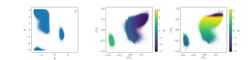
Outline

• Reaction coordinates and free energy computations

• A (short and biased) review of some machine learning approaches for RC

• Free-energy biasing and iterative learning with autoencoders1
       Autoencoders and their training
       Working with free energy weighted distributions
       General presentation of the iterative algorithm
       Illustration/sanity checks on toy examples

• Applications to systems of interest
       Alanine dipeptide
       HSP90 (work in progress)

  1
      soon to be preprinted...
  Gabriel Stoltz (ENPC/Inria)                                Feb. 2021   2 / 27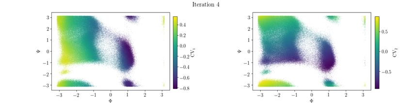
Reaction coordinates
     and free energy computations

Gabriel Stoltz (ENPC/Inria)   Feb. 2021   3 / 27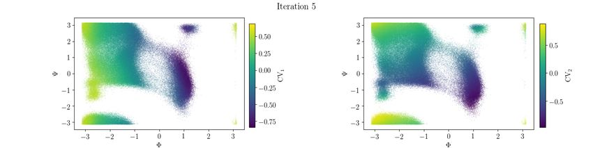
Reaction coodinates (RC) / collective variables (CV)

• Atomic system with positions q = (q1 , . . . , qN ) ∈ D ⊂ RD , Hamiltonian
                  N
                  X   p2i
H(q, p) = V (q) +         , canonical measure Z −1 e−βH(q,p)
                     mi
                            i=1

• Reaction coordinate ξ : RD → Rd with d  D
(ideally such that ξ(qt ) captures the slow part of the dynamics)

• Free energy computed on Σ(z) = {q ∈ RD | ξ(q) = z}
                                                                      !
                                1
                                      Z
                                             −βV (q)
                       F (z) = − ln          e         δξ(q)−z (dq)
                                β     Σ(z)

by various methods (TI, FEP, ABF, metadynamics, etc)2

   2
     Lelièvre/Rousset/Stoltz, Free Energy Computations: A Mathematical Perspective
(Imperical College Press, 2010)
  Gabriel Stoltz (ENPC/Inria)                                             Feb. 2021   4 / 27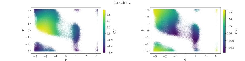
A (short and biased) review of
some machine learning approaches
             for RC

Gabriel Stoltz (ENPC/Inria)   Feb. 2021   5 / 27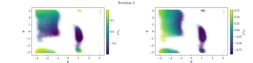
Some representative approaches for finding RC/CV (1)

• Chemical/physical intuition         (distances, angles, RMSDs, coordination numbers, etc)

• Short list of data-oriented approaches                (depending on the data at hand...)

       [supervised learning] separate metastable states
       [unsupervised] distinguish linear models (PCA) and nonlinear ones
       (e.g. based on autoencoders such as MESA3 )
       [dynamics] operator based approaches (VAC, EDMD, diffusion maps,
       MSM; incl. tICA and VAMPNets)
(Huge litterature! I am not quoting precise references here because the list would be too long)

• Other classifications4 possible, e.g. slow vs. high variance CV

   3
     W. Chen and A.L. Ferguson, J. Comput. Chem. (2018); W. Chen, A.R. Tan, and
A.L. Ferguson, J. Chem. Phys. (2018)
   4
     P. Gkeka et al., J. Chem. Theory Comput. (2020)
   Gabriel Stoltz (ENPC/Inria)                                                    Feb. 2021   6 / 27
Some representative approaches for finding RC/CV (2)

  Gabriel Stoltz (ENPC/Inria)                  Feb. 2021   7 / 27
Free-energy biasing and iterative
   learning with autoencoders

Gabriel Stoltz (ENPC/Inria)   Feb. 2021   8 / 27
Autoencoders (1)

  Gabriel Stoltz (ENPC/Inria)   Feb. 2021   9 / 27
Autoencoders (2)
• Data space X ⊆ RD , bottleneck space A ⊆ Rd with d < D

                        f (x) = fdec fenc (x)

where fenc : X →
               − A and fdec : A →
                                − X

Reaction coordinate = encoder part
                                          ξ = fenc

• Fully connected neural network, symmetrical structure, 2L layers

• Parameters p = {pk }k=1,...,K (bias vectors b` and weights matrices W` )

                       fp (x) = g2L [b2L + W2L . . . g1 (b1 + W1 x)] ,

with activation functions g`        (examples: tanh(x), max(0, x), etc)
  Gabriel Stoltz (ENPC/Inria)                                             Feb. 2021   10 / 27
Training autoencoders
• Theoretically: minimization problem in P ⊂ RK
pµ ∈ argmin L(µ, p),
p∈P
with cost function
Z
2
L(µ, p) = Eµ (kX − fp (X)k ) = kx − fp (x)k2 µ(dx)
X
• In practice, access only to a sample: minimization of empirical cost
N N
1 X i 1 X
L(µ̂, p) = kx − fp (xi )k2 , µ̂ = δxi
N N
i=1 i=1
• Typical choices: canonical measure µ, data points xi postprocessed from
positions q (alignement to reference structure, centering, reduction to backbone carbon
atoms, etc)
Gabriel Stoltz (ENPC/Inria) Feb. 2021 11 / 27Training on modified target measures
• Interesting systems are metastable (no spontaneous exploration of phase space)
Sample according to a biased distribution µ e (importance sampling)
• Need for reweighting to learn the correct encoding!
µ(x)
w(x) =
e(x)
µ
• Minimization problem: theoretical cost function
Z
L(µ, p) = kx − fp (x)k2 w(x)e µ(dx),
X
actual cost function
N
X µ(xi )/e
µ(xi )
L(b
µwght , p) = bi kxi − fp (xi )k2 ,
w bi =
w N
i=1
X
µ(xj )/eµ(xj )
j=1
• Only requires the knowledge of µ and µ
e up to a multiplicative constant.
Gabriel Stoltz (ENPC/Inria) Feb. 2021 12 / 27How training is actually performed...
• Gradient descent with minibatching: randomly reshuffle data points,
(r+1)m
1 X
pr = pr−1 − η∇p Lr (pr−1 ), Lr (p) = kxi − fp (xi )k2
m
i=rm+1
One epoch = dN/me gradient steps (in order to visit all the data)
• Actual procedure:
Use keras module in python
Computation of gradient performed with backpropagation
Optimization in fact performed with Adam algorithm
(weights summing to 1 to use default optimization parameters)
“Early stopping” (stop when validation loss no longer improves)
• Many local minima...
Gabriel Stoltz (ENPC/Inria) Feb. 2021 13 / 27Proof of concept (1)
• Gaussian distributions µi = N (0, Σi ) with
1 0 0.01 0
Σ1 = , Σ2 =
0 0.01 0 1
Datasets Di of N = 106 i.i.d. points
• Autoencoders with 2 layers of resp. 1 and 2 nodes, linear activation
functions (' PCA)
• Training on:
D1
D2
D2 with reweighting w
bi ∝ µ1 /µ2
Gabriel Stoltz (ENPC/Inria) Feb. 2021 14 / 27Proof of concept (2)
Heat maps of fenc
D1 D2 , Unweighted D2, Reweighted
1.0
1.0
0.5 0.8
Encoder Variable
0.6
x2
0.0
0.4
−0.5 0.2
−1.0 0.0
−1 0 1 −1 0 1 −1 0 1
x1 x1 x1
Third encoder very similar to the first: projection on x1 .
Second encoder projects on a direction close to x2 .
Gabriel Stoltz (ENPC/Inria) Feb. 2021 15 / 27Proof of concept with free energy biasing (1)
Two dimensional potential (“entropic switch”)5
−x21 −(x2 −1/3)2 −(x2 −5/3)2
V (x1 , x2 ) = 3e e −e
2
2 2
− 5e−x2 e−(x1 −1) + e−(x1 +1) + 0.2x41 + 0.2(x2 − 1/3)4
p
Trajectory from q j+1 = q j − ∇V (q j )∆t + 2β −1 ∆tGj for β = 4 and
∆t = 10−3 −→ metastability in the x1 direction
5
S. Park, M.K. Sener, D. Lu, and K. Schulten (2003)
Gabriel Stoltz (ENPC/Inria) Feb. 2021 16 / 27Proof of concept with free energy biasing (2)
• Free energy biasing: distributions Zi−1 exp (−β [V (q) − Fi (ξi (q))])
Z Z
1
F1 (x1 ) = − ln e−βV (x1 ,x2 ) dx2 , F2 (x2 ) = −β −1 ln ... dx1
β R R
Three datasets: unbiased trajectory, trajectories biased using F1 and F2
(free energy biased trajectories are shorter but same number of data points N = 106 )
• Autoencoders: 2-1-2 topology, activation functions tanh (so that RC is
in [−1, 1]) then identity
• Five training scenarios:
training on long unbiased trajectory (reference RC)
ξ1 -biased trajectory, with or without reweighting
ξ2 -biased trajectory, with or without reweighting
Gabriel Stoltz (ENPC/Inria) Feb. 2021 17 / 27Proof of concept with free energy biasing (3)
Unweighted Training Weighted Training
2.5
1.0
2.0
0.8
Encoder Variable
Normalize to compare 1.5
0.6
1.0
x2
0.5 0.4
min
ξAE (x) − ξAE
norm 0.0
ξAE (x) = max min
0.2
ξAE − ξAE −0.5
0.0
−1.0
−2 −1 0 1 2 −2 −1 0 1 2
x1 x1
Unbiased training
2.5
2.0
1.0
x1 -biased trajectory
0.8
Encoder Variable
1.5
0.6
1.0 Unweighted Training Weighted Training
2.5
x2
0.5 1.0
0.4
0.0
2.0
0.2 0.8
Encoder Variable
−0.5 1.5
−1.0 0.0 1.0 0.6
−2 −1 0 1 2
x2
x1
0.5 0.4
Reference RC 0.0
0.2
−0.5
(distinguishes well the 3 wells) 0.0
−1.0
−2 −1 0 1 2 −2 −1 0 1 2
x1 x1
x2 -biased trajectory
Gabriel Stoltz (ENPC/Inria) Feb. 2021 18 / 27Full iterative algorithm (Free Energy Biasing and Iterative Learning with AutoEncoders)
Input: Initial condition q0 , autoencoder topology and initialization parameters Ainit , number of
samples N , simulation procedure S and adaptive biasing procedure SAB , maximum number of
iterations Imax , minimum convergence score smin
Initialization
Sample traj0 ← S(q0 , N )
Initialize autoencoder AE0 ← Ainit
Train AE0 on traj0 with weights (w b0 , . . . , w
bN ) = (1, . . . 1)
Extract the encoder function ξ0 : x 7→ ξ0 (x)
Iterative update of the reaction coordinate
Set i ← 0, s ← 0
While i < Imax and s < smin Treshold smin to be determined
Set i ← i + 1
Sample traji , Fi ← SAB (q0 , N, ξi−1 ) in our case: extended ABF
j
Compute weights w bj ∝ e−βFi (ξi−1 (x ))
Initialize autoencoder AEi ← Ainit
Train AEi on traji with sample weights w bj
Extract the encoder function ξi : x 7→ ξi (x)
Set s ← regscore(ξi−1 , ξi ) Convergence metric to be made precise
Set ξfinal ← ξi
Production of output:
Sample trajfinal , Ffinal ← SAB (q0 , Nfinal ξfinal ) with Nfinal large enough to ensure PMF convergence
Gabriel Stoltz (ENPC/Inria) Feb. 2021 19 / 27Discussion on the convergence criterion
• Check convergence of CV?
Quantify ξi ≈ Φ(ξi−1 ) for some monotonic function Φ
• Approach: approximate Φ by a linear model → linear regression
• Regression score between ξ and ξ 0
Two sets of values of RC (ξ(q 1 ), . . . , ξ(q N )) and (ξ 0 (q 1 ), . . . , ξ 0 (q N ))
Match them with a linear model M (z) = W z + b
N
X 2
ξ 0 (q i ) − M (ξ(q i ))
i=1
Coefficient of determination R2 = 1 − N
2
ξ 0 (q i ) − ξ¯0
X
i=1
Maximization of R2 w.r.t. W, b provides regscore(ξ 0 , ξ)
• Value of smin computed using some bootstrap procedure
Gabriel Stoltz (ENPC/Inria) Feb. 2021 20 / 27The iterative algorithm on the toy 2D example
Left: with reweighting
Convergence to RC ' x1
Right: without reweighting
No convergence
(cycles between two RCs)
Gabriel Stoltz (ENPC/Inria) Feb. 2021 21 / 27Applications to systems of interest Gabriel Stoltz (ENPC/Inria) Feb. 2021 22 / 27
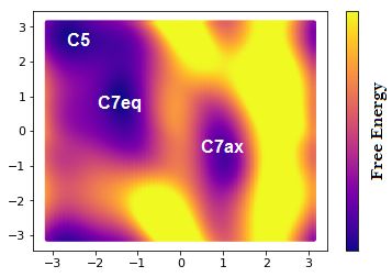
Alanine dipeptide
• Molecular dynamics:
openmm with openmmplumed to link it with plumed
colvar module for eABF and computation of free energies
timestep 1 fs, friction γ = 1 ps−1 in Langevin dynamics

• Machine learning:
keras for autoencoder training
input = carbon backbone (realignement to reference structure and centering)
neural network: topology 24-40-2-40-24, tanh activation functions

  Gabriel Stoltz (ENPC/Inria)                                             Feb. 2021   23 / 27
Ground truth computation
Long trajectory (1.5 µs), N = 106 (frames saved every 1.5 ps)
RC close to dihedral angles Φ, Ψ

Quantify smin = 0.99 for N = 105 using a bootstraping procedure

For the iterative algorithm: 10 ns per iteration
(compromise between times not too short to allow for convergence of the free energy, and not
too large in order to alleviate the computation cost)

   Gabriel Stoltz (ENPC/Inria)                                                 Feb. 2021   24 / 27
Results for the iterative algorithm

 iter.    regscore      (Φ, Ψ)
   0         −           0.922
   1       0.872         0.892
   2       0.868         0.853
   3       0.922         0.973
   4       0.999         0.972
   5       0.999         0.970
   6       0.999         0.971
   7       0.999         0.967
   8       0.998         0.966
   9       0.999         0.968

  Gabriel Stoltz (ENPC/Inria)         Feb. 2021   25 / 27
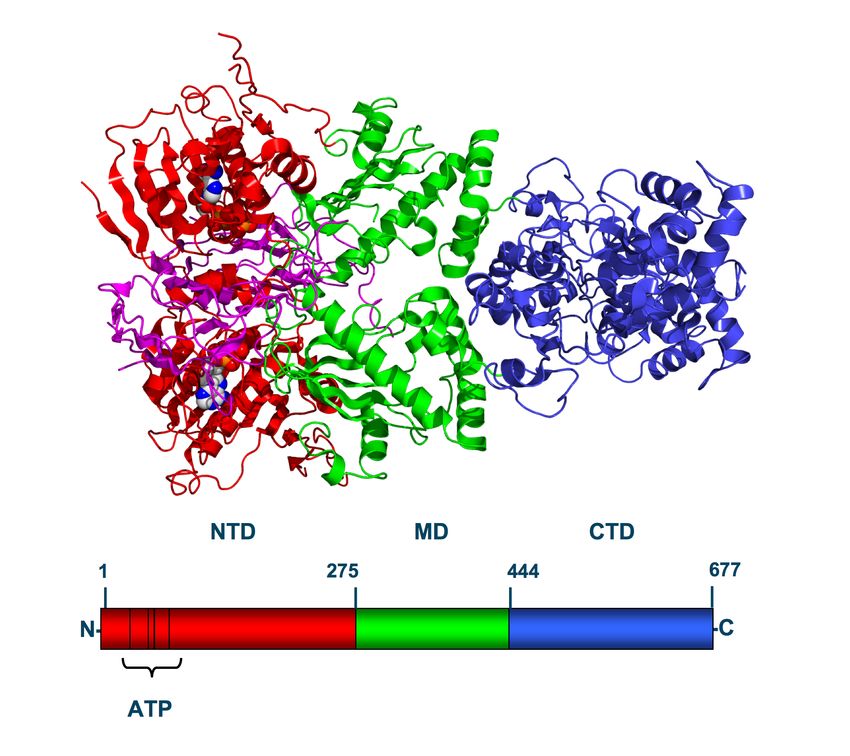
HSP90 (work in progress...)
Chaperone protein
assisting other
proteins to fold
properly
(incl. proteins
involved in tumor
growth)
−→ look for inhibitors
(e.g. targeting binding
region of ATP)
(picture from https://en.wikipedia.org/wiki/File:Hsp90 schematic 2cg9.png)
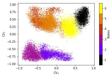
Gabriel Stoltz (ENPC/Inria) Feb. 2021 26 / 27HSP90 (work in progress...) 6 conformational states, data from 10 × 20 ns trajectories, input features = 621 C carbons, AE topology 621-100-5-100-621 Gabriel Stoltz (ENPC/Inria) Feb. 2021 27 / 27
You can also read