Impact du brûlage in-situ sur la qualité de l'air - Cedre
←
→
Page content transcription
If your browser does not render page correctly, please read the page content below
Impact du brûlage in-situ sur la qualité de
                    l’air

      Laurence ROUÏL ,
      Head of the « Environmental modelling and decision making » department,
      Laurence.rouil@ineris.fr

            Institut National de l’Environnement Industriel et des Risques

20ième journée d’information du CEDRE , Paris, Mars 2015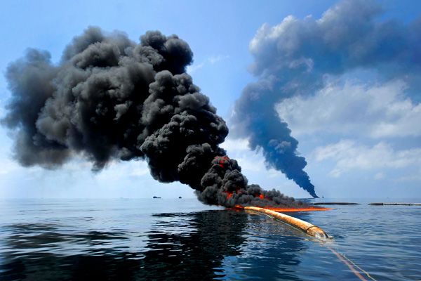
Le brûlage in-situ : une source importante de polluants atmosphériques

•   Comme les feux industriels, brûlages de torchères,
    ou même les feux de forêts, le brûlage in-situ
    est à l’origine d’émissions dans l’atmosphère de
    quantités massives de polluants atmosphériques.
•   L’impact environnemental et sanitaire dépend de la
    localisation du feux, des conditions de brûlage, des
    conditions météorologiques mais influence toujours
    la qualité de l’air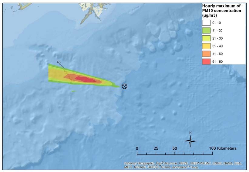
Quels sont les polluants émis
                                                            - Oxydes d’azotes
                                                            - Particules (PM10 et                                                75
                                                            PM2.5)                                                                                                 CO2
                                                            - Dioxyde de soufre
                                                                                                                                                                   H2O
                                                            - hydrocarbures (VOC)
                                                            - Hydrocarbures                                                                                 12     CO
                                                            aromatiques
                                                                                                                                                      3
                                                            polycycliques (PAHs)                                                           10                      Other (PAHs, VOC,
                                                            - dioxines                                                                                             NOx, ..)

                                                                                                                                                      0,2

     (adapted from SL Ross Environmental Research Ltd, 2010).                                                                         (adapted from Tennyson, 1994, Buist, 1999)

                           Constituent                                                    Quantity Emittedb
                                                                                      (g emission/kg oil burned)
                 Carbon Dioxide (CO2)                                                            3000                                      20 g/kg
               Particulate Matter (PM)                                                        50 – 200c,d
                Elemental Carbon (EC)                                                           4 – 10e                                    0.5 g/kg
                 Organic Carbon (OC)                                                           45 – 90e
               Carbon Monoxide (CO)                                                             20 – 50
                Nitrogen Oxides (NOx)                                                              1                                       2.5 g/kg
                  Sulfur Dioxide (SO2)                                                             3e                                      0.5- 1 g/kg
         Volatile Organic Compounds (VOC)                                                          5
      Polynuclear Aromatic Hydrocarbons (PAH)                                                    0.004
aUpdated  from Buist et al., 1994, based on the Kuwait pool fire (Allen and Ferek, 1993) and the NOBE data (Ross et al., 1996)
bQuantities will vary with burn efficiency and composition of parent oil.                                                        Facteurs d’émission associés aux feux de forêts,
cFor crude oils soot yield = 4 + 3 lg(fire diameter); yield in mass %, fire diameter in cm (Fraser et al., 1997)
                                                                                                                                 d’après Turquety et al, 2013
dEstimates published by Environment Canada are considerably lower, ca. 0.2% to 3% for crude oil (Fingas, 1996)

efrom Ross et al., 1996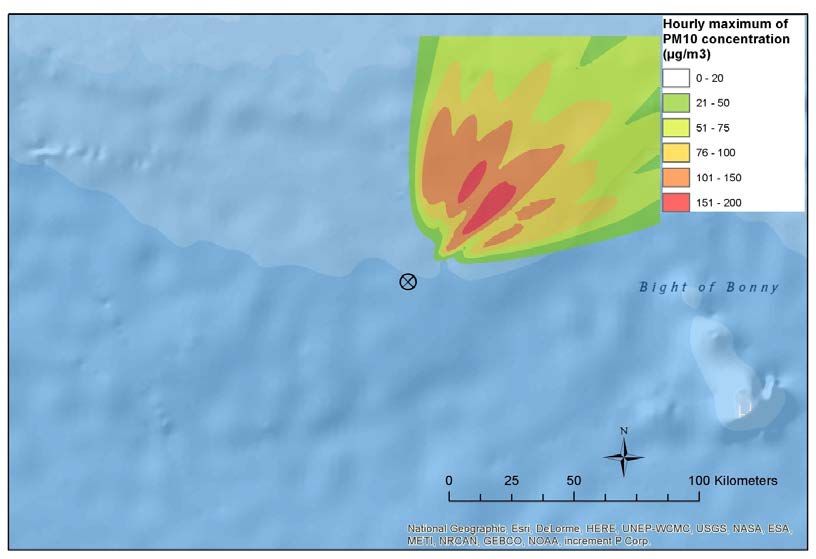
ISB versus other types of emissions Total PM10 emission during DWH : 40 Kton Total PM10 emission in the USA : 600Kton Buncefield PM10 emissions : 10Kton Total black carbon released during DWH: 100-200 Ktons Total elemental carbon : 8000 Kton during the Kuwait fires CO emissions during DWH : 104 tons CO emissions during the 2010 russian forest fires: 19x106–33 x106 tons
EU Air quality standards ( AQ Directive)

  Pollutants   AQ Directive 2008/50/EC
  PM10         50 µg/m3 daily average not exceeded more than 35 fois/year
               40 µg/m3 yearly average
  PM2.5        Exposure index based on the daily average
               25 µg/m3 yearly average (20µg/m3 in 2020)
  O3           120 µg/m3 8-hours average not exceeded more than 25 days/year

  NO2          40 µg/m3 yearly average
               200 µg/m3 hourly average not exceeded more than 18 times/year
  SO2          350 µg/m3, hourly average not exceeded more than 18 times/year
               125 µg/m3 daily average not exceeded more than 5 fois/year
  Lead (Pb)    0.5 µg/m3 yearly average

  Benzene      5 µg/m3 yearly average
  (C6H6)
  CO           10 mg/m3 maximum 8-hours daily average
US Air quality standards (Clean Air Act)
                Pollutant                               Primary/Secondary                              Averaging time                                           Level                                                     Form

                                                                                                      8 hour                              9 ppm                                                     Not to be exceeded more than
  Carbon Monoxide (CO)                              Primary
                                                                                                      1 hour                              35 ppm                                                    once per year
                                                                                                      Rolling 3 month
  Lead (Pb)                                         Primary and secondary                                                                 0.15 µg m-3 (a)                                           Not to be exceeded
                                                                                                      average
                                                                                                                                                                                                    98th percentile, averaged over 3
                                                    Primary                                           1 hour                              100 ppb
  Nitrogen Dioxide (NO2)                                                                                                                                                                            years
                                                    Primary and secondary                             1 year                              53 ppb (b)                                                Annual Mean
                                                                                                                                                                                                    Annual fourth-highest daily
  Ozone (O3)                                        Primary and secondary                             8 hour                              75 ppb (c)                                                maximum 8-hr concentration,
                                                                                                                                                                                                    averaged over 3 years
                                                    Primary                                                                               12 µg m-3                                                 Annual mean, averaged over 3
                                                                                                      1 year
                                                    secondary                                                                             15 µg m-3                                                 years
  Particles PM2.5
                                                                                                                                                                                                    98th percentile, averaged over 3
                                                    Primary and secondary                             24 hours                            35 µg m-3
                                                                                                                                                                                                    years
                                                                                                                                                                                                    Not to be exceeded more than
  Particles PM10                                    Primary and secondary                             24 hours                            150 µg m-3                                                once per year on average over 3
                                                                                                                                                                                                    years
                                                                                                                                                                                                    99th percentile of 1-hour daily
                                                    Primary                                           1 hour                              75 ppb (d)                                                maximum concentrations,
                                                                                                                                                                                                    averaged over 3 years
  Sulfur Dioxide (SO2)
                                                                                                                                                                                                    Not to be exceeded more than
                                                    Secondary                                         3 hours                             0.5 ppm
                                                                                                                                                                                                    once per year

  (a) Final rule signed October 15, 2008. The 1978 lead standard (1.5 µg/m3 as a quarterly average) remains in effect until one year after an area is designated for the 2008 standard, except that in areas designated nonattainment for the 1978, the
  1978 standard remains in effect until implementation plans to attain or maintain the 2008 standard are approved.

  (b) The official level of the annual NO2 standard is 0.053 ppm, equal to 53 ppb, which is shown here for the purpose of clearer comparison to the 1-hour standard.

  (c) Final rule signed March 12, 2008. The 1997 ozone standard (0.08 ppm, annual fourth-highest daily maximum 8-hour concentration, averaged over 3 years) and related implementation rules remain in place. In 1997, EPA revoked the 1-hour
  ozone standard (0.12 ppm, not to be exceeded more than once per year) in all areas, although some areas have continued obligations under that standard (“anti-backsliding”). The 1-hour ozone standard is attained when the expected number of
  days per calendar year with maximum hourly average concentrations above 0.12 ppm is less than or equal to 1.

  (d) Final rule signed June 2, 2010. The 1971 annual and 24-hour SO2 standards were revoked in that same rulemaking. However, these standards remain in effect until one year after an area is designated for the 2010 standard, except in areas
  designated nonattainment for the 1971 standards, where the 1971 standards remain in effect until implementation plans to attain or maintain the 2010 standard are approved.
Evaluer l’impact sanitaire de l’in-situ burning
• Critère généralement utilisé : respect des normes de qualité de l’air, notamment pour les
particules (PM10 et PM2.5)
• Besoin d’évaluer l’impact du panache sur les concentrations de polluants atmosphériques
dans les zones potentiellement impactées pour limiter l’exposition des populations
• Possibilité de réaliser de campagnes de mesures pour surveiller la qualité de l’air pendant
les opérations
• Mise en œuvre de modèle pour prédire les effets et les distances « de sécurité » .
Exemple : table établie à partir de simulations du logiciel ALOFT
1 mile = 1.6 km
Distance de sécurité entre les feux et les populations sous le vent, d’après le guide ARRT (Alaska Regional respose Team)Marine conditions for atmospheric dispersion
Atmospheric dispersion is driven by the nature of the surface. Sea surface implies different
dispersion conditions compared to soils
Lower boundary layer heights (more stable conditions), the sea surface temperature
being lower than the temperature in the air
Stable conditions when burning
High relative humidity
Presence of sea salts (potential interactions but not studied so far)
Sea temperature drives the air temperature (min temperature in March, max in
September)
In certain areas (Artic region) the temperature of the sea can lead to high gradients with the
atmosphere, with very low boundary layer heights
LIDAR measurement
Plume center
Newfoundland Offshore Burn Experiment (NOBE, 1993)
University of WashingthonEvaluer l’impact sanitaire de l’in-situ burning
• Critère généralement utilisé : respect des normes de qualité de l’air, notamment pour les
particules (PM10 et PM2.5)
• Besoin d’évaluer l’impact du panache sur les concentrations de polluants atmosphériques
dans les zones potentiellement impactées pour limiter l’exposition des populations
• Possibilité de réaliser de campagnes de mesures pour surveiller la qualité de l’air pendant
les opérations
• Mise en œuvre de modèle pour prédire les effets et les distances « de sécurité » .
Exemple : table établie à partir de simulations du logiciel ALOFT
1 mile = 1.6 km
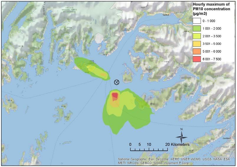
Distance de sécurité entre les feux et les populations sous le vent, d’après le guide ARRT (Alaska Regional respose Team)Etude de sensibilité Scenario #1: Alaska coast (60°48”36’N / 146°52”23’W) Date of spill : 09/11/2014 07:30:00 Water temperature : 8°C Scenario #2: Gulf of Mexico (28°11”59’N / 88°47”59’W) Date of spill: 14/09/2014 11:00:00 Water temperature : 20°C Scenario #3: West African Coast (3° 01′ N / 6° 58′ E) Date of spill : 09/11/2014 07:00:00 Water temperature: 28°C 7 days of simulation; same source term Gaussian model : ADMS run by INERIS
Results: maximum hourly PM10 concentrations

                                             Gulf of mexico

 Alaska Coast

                             West African Coast
Analyse :
• Une certaine variabilité dans les résultats qui ne permet pas d’assurer la validité des
distances de sécurité tabulées par ARRT
• Grande sensibilité aux conditions météorologiques, les précipitations et la
température de l’eau
• Pas de simulation des transformations chimiques, bien que :
Massive release of VOC can impact ozone concentrations of ozone
concentrations downwind the plume
For the same reason ISB can favour secondary organic aerosol formation, and
therefore increase PM concentrations
Long range transport of a pollutants in the plume is a main driverConclusions
• Relativement peu d’études d’impact du brûlage in-situ sur la qualité de l’air : plutôt
réalisées avec des modèles simples en vue d’une évaluation des distances d’impact.
Name Type of study Modelling tools Reference
Deepwater Horizon (2010) Risk assessment levels Plume model (AERMOD) Schaum et al.,
due to dioxine 2012
+
(PCDD/PCDF) emission
Regional study using HYSPLIT
model in an eulerian/puff mode
-
plume rise computation from
OBODM (Dumbauld et al.
(1973) derivation of Briggs formula
(1971), for large source)
NOBE and Alaskan plume Trajectory and particle LES particle model (ALOFT-FT and Mc Grattan et al.,
(Burning of emulsion test) concentration simulation ALOFT-CT) 1996
MOBILE Mesoscale Trajectory and particle LES particle model (ALOFT-FT) Walton et al.,
experiment concentration simulation 1993
NOBE, ALASKA and Trajectory and particle Sum - up of previous papers + Mc Grattan et al.,
MOBILE concentration simulation comparison with CALPUFF 2003
Coastal measurement in Simulation of emissions Plume model + specific adaptation Hanna et al.,
California and Gulf of from offshore sources, not for over sea emission and coastal 1985
Mexico specific to in-situ burning. environment• Mais il est difficile de qualifier l’impact du brulage in-situ sur l’environnement sans
prendre en compte des facteurs particulier liés à la localisation, les conditions
météorologiques, voire la nature des produits brûlés
• Néanmoins certaines campagnes de brulage instrumentées permettent d’accéder à
de nouvelles données
Deepwater Horizon (DWH) oil spill : Middlebrook et al., 2011 predicted high
Secondary Organic Aerosols along the coast
Impact of the evaporation of VOC on O3 production (some papers)
• Importance potentielle des impacts des retombées de poussières, carbone suie (sur
le continent Articque?), dioxines et HAPS à cause de leurs effets sur la santé. Le
dépôt est faible en mer met peut être significatif sur terre là où vivent les populations.You can also read