Incorporating Scenario Analysis into the Federal Reserve's Policy Strategy and Communications
←
→
Page content transcription
If your browser does not render page correctly, please read the page content below
Incorporating Scenario Analysis into the
                    Federal Reserve’s Policy Strategy and Communications*

                          Michael Bordo, Andrew Levin, and Mickey Levy

                                  Economics Working Paper 20108

                                         HOOVER INSTITUTION
                                          434 GALVEZ MALL
                                        STANFORD UNIVERSITY
                                      STANFORD, CA 94305-6010

                                               June 2020

The U.S. economy currently faces a truly extraordinary degree of uncertainty as a consequence
of the COVID-19 pandemic. Consequently, the Federal Reserve should begin highlighting
alternative scenarios that illustrate key risks to the economic outlook, and those scenarios
should inform the Fed’s policy strategy and public communications. We present a set of
illustrative scenarios, including a baseline scenario with a rapid but incomplete recovery later
this year (an upward-tilting checkmark), a benign scenario in which the rapid dissemination of
an effective cure or vaccine generates a rapid v-shaped recovery, and a severely adverse scenario
involving extraordinarily high and persistent unemployment and the onset of deflation. Insights
into these scenarios can be drawn from key historical episodes, including the Spanish flu,
the Great Depression, the end of World War II, and the global financial crisis. We conclude
by identifying key challenges that the Federal Reserve will need to address in adjusting its
monetary policy and emergency credit facilities under these three alternative scenarios.
Keywords: COVID-19 pandemic, monetary policy, lender of last resort programs.
JEL Codes: E52, E58, N11, N12.

The Hoover Institution Economics Working Paper Series allows authors to distribute research for
discussion and comment among other researchers. Working papers reflect the views of the
authors and not the views of the Hoover Institution.

*
  Bordo is a professor of economics at Rutgers University, director of the Center for Monetary and
Financial History, a research associate of the National Bureau of Economic Research (NBER), and a
Distinguished Visiting Fellow at the Hoover Institution, Stanford University. Levin is a professor of
economics at Dartmouth College, research associate of the NBER, and international research fellow of the
Centre for Economic Policy Research. Levy is chief economist for the Americas and Asia at Berenberg
Capital Markets LLC. All three coauthors are members of the Shadow Open Market Committee. Roiana
Reid was very helpful in contributing to the preparation of this paper. The views expressed here are solely
those of the authors and do not represent the views of any other person or institution.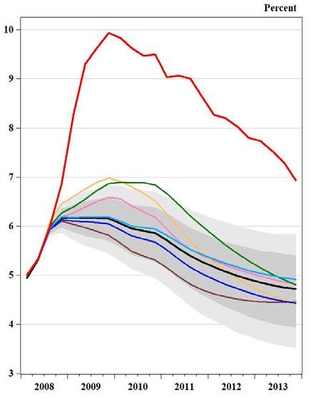
1. Introduction

The U.S. economy is beginning to reopen after undergoing a catastrophic disruption due to
the COVID-19 pandemic and government shutdowns. Retail sales (excluding food) in April
were nearly 30 percent lower than in February, and millions of Americans have lost their jobs,
resulting in an extremely high unemployment rate of nearly 15 percent. Moreover, even that rate
understates the total damage to the job market. All told, the recent collapse in economic activity
has been reminiscent of the Great Depression but within a timeframe of weeks instead of years.

Looking forward, the uncertainty about the U.S. economic outlook is extraordinarily high,
reflecting a very wide range of potential trajectories for the COVID-19 pandemic. A rapid
recovery in economic activity and employment to pre-pandemic levels is possible, particularly
if the accelerated development of vaccinates and/or antiviral medicines bears fruit. However,
public health experts have cautioned that a much longer time horizon might be required to
obtain an effective vaccine or cure for the virus; in that case, even with the lifting of quarantine
measures, many individuals might continue to engage in voluntary social distancing, leading to
a more severe and protracted economic downturn.

Since the onset of the COVID-19 pandemic, the Federal Reserve has acted promptly and
forcefully in carrying out its role as lender of last resort, taking unprecedented actions to
avoid a financial crisis and sustain the supply of credit. With fiscal backing from the
Congress and the U.S. Treasury, the Federal Reserve has launched emergency liquidity facilities
that have prevented the pandemic from triggering a systemic financial crisis. The Fed is now
conducting outright purchases of corporate securities (including bonds commonly classified as
“junk”), direct lending to businesses, and purchases of state and municipal debt.

The Federal Reserve’s monetary policy actions have also been extraordinary. During the
first half of March, the Federal Open Market Committee (FOMC) reduced the target federal
funds rate to zero and indicated that monetary policy will remain accommodative until the
economy is back on track. Since that time, the FOMC has purchased about $2 trillion in Treasury
securities and agency mortgage-backed securities (MBS), and its balance sheet now exceeds
$7 trillion. With the short end of the yield curve pinned near zero, these actions have had only
muted effects on longer-term Treasury yields, which serve as a benchmark for other credit rates;
the 10-year Treasury yield is currently about 0.9 percent, less than half a percentage point below
its end-February level.

Clarity about the Federal Reserve’s policy strategy is essential for mitigating the economic
and financial consequences of the COVID-19 pandemic. As America’s central bank, the
Federal Reserve is responsible for carrying out its mandate of fostering maximum employment
2
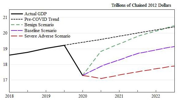
Figure 1: Illustrative Scenarios for the Trajectory of Real GDP
Source: U.S.Bureau of Economic Analysis, authors’ calculations
and price stability as well as promoting the stability of the financial system. Its policy tools are
now directly aimed at facilitating the supply of credit to households and businesses as well as
states and municipalities. Consequently, the Fed’s communications are crucial for sustaining
public confidence and fostering the recovery.
In these circumstances, the Federal Reserve should start explaining its policy strategy by
referring to alternative scenarios rather than focusing on a single benchmark projection.
The extraordinary degree of uncertainty cannot be conveyed merely by including “fan charts”
around a baseline projection. Rather, the Federal Reserve should identify key risks to the
economic outlook, formulate alternative scenarios to illustrate those risks, and explain its plans
for mitigating and addressing those risks.
In this note, we show how this approach can be implemented by describing the broad contours of
a baseline projection that is bracketed by two plausible alternative scenarios. Figure 1 illustrates
this approach for the trajectory of real GDP under the following three scenarios:
(1) In the baseline scenario, the U.S. economy exhibits a partial rebound this year, mainly
reflecting re-employment in construction, manufacturing, and a portion of service-producing
industries. Nonetheless, employment remains far below its pre-pandemic peak and recovers
only slowly over coming years, while inflation remains well below the Fed’s target.
(2) In the benign scenario, medical researchers develop an effective and widely available
vaccine or cure, ending the pandemic and restoring confidence. Consequently, a robust recovery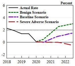
3

fosters rapid growth in economic activity and employment, and the economy returns close to
its pre-pandemic trend path by the middle of next year.

(3) In the severe adverse scenario, no effective vaccine or cure becomes available, and the threat
of infection does not abate. Consequently, consumer and business sentiment wanes further,
leading to sustained high unemployment, further business closures and widespread credit
defaults, thereby triggering an adverse feedback loop between the real economy and the financial
system as well as persistent deflationary pressures.

We provide additional perspective on these scenarios in light of several relevant historical
episodes, including the Spanish flu pandemic of 1918-19, the Great Depression of the 1930s,
and the economic transition at the end of World War II. We then highlight the distinct policy
challenges that the Federal Reserve will face in adjusting its monetary policy and emergency
credit facilities under these three alternative scenarios. For example, in the benign scenario,
the Fed might need to unwind its emergency actions very rapidly to avoid an undesired credit
boom or undesired high inflation as in the wake of World War II. Conversely, in the severe
adverse scenario, the Fed would be at a crossroads of either expanding its monetary toolbox
or remaining on the sidelines as it did in the Great Depression.

2. The Rationale for Alternative Scenarios

The Federal Reserve now faces the challenge of making crucial policy decisions amid an
unprecedented degree of uncertainty. Unlike normal periods, this uncertainty hinges on medical
and public health concerns that are well beyond the scope of the Fed’s monetary policy and that
cannot be captured by conventional macroeconomic modeling. In the face of such extreme
uncertainty, the Federal Reserve must weigh the relative benefits of its actions, including
potentially unintended consequences and longer-run risks.

In effect, Fed officials are analogous to a team of physicians, where the patient is the U.S.
economy. In a complex medical situation, the patient needs a team of expert doctors, who
examine an array of information to determine the appropriate course of treatment. That process
involves extensive consultations with the patient and the patient’s family to discuss the medical
diagnosis, treatment plans, uncertainties, risks, and contingency plans. Such consultations need
to be managed carefully to facilitate clear communications without unnecessarily alarming the
patient. The Fed should start engaging in similar consultations with the public and in its reports
to Congress (which is the Fed’s boss).

The Federal Reserve currently frames its monetary policy in terms of a single benchmark
projection of the economy, namely, the median of FOMC participants’ individual assessments of
the most likely trajectory for key macroeconomic indicators, including real GDP growth, the
unemployment rate, headline inflation for personal consumption expenditures (PCE), core PCE
4

inflation, and the federal funds rate. 1 These projections are released each quarter at the same time
as the FOMC meeting statement and are then discussed at the Fed chairman’s press conference,
with further details published three weeks later in the Summary of Economic Projections (SEP)
that accompanies the FOMC minutes. 2

These SEP projections reflect each FOMC participant’s individual judgment regarding the
appropriate path of monetary policy. The chart showing the distribution of their assessments for
the federal funds rate is commonly known as the “dot plot.” However, the SEP does not include
any projections for the size and composition of the Fed’s balance sheet, even though the FOMC
highlights balance sheet operations as a key element of its monetary toolbox.

The SEP conveys uncertainty about the economic outlook by reporting on FOMC participants’
qualitative assessments about whether or not that uncertainty is elevated relative to “normal” and
whether the risks to the outlook are judged to be “balanced”, “tilted to the upside”, or “tilted to
the downside.” The SEP also includes tabulations of historical forecast errors for each key
macroeconomic indicator; these tabulations are often referred to as “fan charts.”

This focus on a single benchmark projection is not satisfactory for framing the Fed’s policy
strategy and contingency plans, especially amid current heightened risks and uncertainties.
Rather, the Federal Reserve should engage in scenario analysis aimed at identifying specific
risks to the economic outlook, and it should formulate and communicate its contingency plans
for addressing those risks. 3 Since the financial crisis of 2008-2009, the Fed has conducted annual
stress tests of the largest financial institutions, and these evaluations have proven helpful for
gauging each institution’s capacity for coping with a severe adverse scenario and ensuring that it
has a well-designed strategy for doing so.

The Fed’s policy deliberations and communications would benefit from engaging in stress
tests of its own policy strategy and contingency plans. Scenario analysis is particularly
advantageous when uncertainty is extraordinarily high due to factors that are not well captured
by conventional econometric or statistical methods. In such circumstances, assigning definite
probabilities to each of the plausible outcomes may not be practical. Economists commonly
describe such circumstances as Knightian uncertainty, while others have simply referred to the
“unknown unknowns.” 4 Lord Mervyn King has recently coined the term radical uncertainty and
has specifically advocated that central banks should utilize a narrative approach to strategic

1
  The voting members of the FOMC include the governors of the Federal Reserve Board, the president of the New
York Fed, and four of the other eleven Federal Reserve Bank presidents (who have voting membership on an annual
rotating basis). However, SEP projections are submitted by all of these FOMC participants, including those who are
not currently voting members.
2
  For each of these macroeconomic indicators, the Fed publishes the range of projections across FOMC participants
and a “central tendency” interval that is calculated by excluding the highest three and the lowest three projections.
3
  See Levin (2014, 2015) and Levy (2019).
4
  See Knight (1921) and Hansen and Sargent (2007). The phrase “known unknowns and unknown unknowns” was
popularized by U.S. Secretary of Defense Donald Rumsfeld at a news briefing in 2002.
5

planning and public communications in such circumstances; similarly, Nobel Prize winner
Robert Shiller has highlighted the importance of narratives in determining major economic
outcomes. 5

Some officials might worry that more transparent risk assessments and contingency plans could
undermine public confidence. But the health care analogy is helpful here: in a serious medical
situation, the patient can easily imagine worst-case outcomes and become unduly anxious,
confused, or depressed, and that stress tends to exacerbate the patient’s condition. Therefore, an
effective medical team consults carefully with the patient and the patient’s family, and those
consultations are conducive to better health outcomes and help speed the patient’s recovery.

Similar lessons are evident from national defense and hurricane preparedness. In a military
context, scenario analysis (informally known as “war games”) have long played a key role in
strategic planning. In that context, the analysis is closely held to protect sensitive national
security information. By contrast, when meteorologists identify an incipient hurricane, weather
forecasters give regular updates to the public about the range of potential trajectories implied by
alternative forecasting models, and such information facilitates public preparedness and helps
mitigate the extent of damage from the hurricane itself.

Some officials might also worry that publishing alternative scenarios could unduly constrain the
Fed’s policy flexibility. In practice, however, it will be readily apparent that such scenarios are
intended to be illustrative rather than serving as binding commitments. The set of illustrative
alternatives and the specific contours of each scenario can be updated regularly in light of
incoming information, following essentially the same process that the FOMC currently uses in
producing and publishing its quarterly outlook. Moreover, policymakers can easily highlight or
downplay any particular scenario as its relative likelihood changes over time.

Moreover, scenario analysis does not constrain the Federal Reserve to follow any fixed strategy
or rule. Rather, this approach would facilitate the Fed’s policy deliberations and enhance the
clarity of its public communications. Indeed, explaining its policy strategy clearly would help
foster public confidence far more than following its conventional approach of making decisions
on a “meeting-by-meeting” basis.

Thus, once per quarter, the Fed should formulate and publish a set of alternative scenarios
along with its baseline SEP projection. In addition to the macroeconomic variables currently
included in the SEP, each scenario should indicate the Fed’s assessment of appropriate monetary
policy under that scenario. These assessments should include the anticipated trajectory for the
overall size and composition of the Fed’s balance sheet, especially since the federal funds rate is
currently anchored near zero and the Fed is engaged in open-ended asset purchases. The broad

5
    See Shiller (2019) and Kay and King (2020).
6 contours of these alternative scenarios can be presented at the Fed chair’s press conference, with further details disseminated in the SEP three weeks later. To facilitate the effectiveness of this approach, it will be crucial for the Federal Reserve to foster and sustain a work environment that encourages openness and outside-the-box thinking. Such an environment will strengthen the Fed’s ability to identify material risks to the economy and the financial system and to formulate strategic plans for avoiding or mitigating such risks. 3. Illustrative Scenarios To help visualize how our proposed approach could be implemented, we now characterize the contours of a baseline scenario bracketed by two plausible alternative scenarios. The quantitative features of these scenarios are reported in Table 1 and are shown in Figures 2 and 3 as well as in Figure 1 above. 3.1 Baseline Scenario Our baseline forecast of a moderate recovery assumes that the government manages a gradual, successful reopening of the economy, with ongoing limitations on public events and social distancing rules. While increasingly reliable testing for covid-19 gradually become more widely available, no effective vaccine or antiviral treatment becomes available before 2022. As a consequence, consumer and business confidence remain cautious, which contributes to a higher rate of personal saving and constrained business spending. The shape of this economic recovery appears like an upward-tilted checkmark, with a sharp but incomplete rebound during the second half of 2020, followed by more gradual pace of recovery thereafter. Consequently, real GDP does not return to its pre-pandemic level until late 2022. After reaching a peak of around 15 percent, the unemployment rate is projected to recede to about 10 percent by the end of this year and declines more slowly to about 6½ percent by the end of 2022. Consumer spending, residential investment, and government purchases are the key drivers at the initial stages of recovery, while business fixed investment and exports lag substantially. These trends will be accompanied by a tilt away from globalization and mounting constraints on international capital flows. Headline inflation turns negative and involves a temporary deflation reflecting the sharp decline in oil prices and downward pressure on prices of other goods and services during the sharp economic contraction, while core inflation goes to zero. The recovery in oil prices eliminates deflation but the core PCE price index remains close to zero (price stability) early in the recovery. Market and survey-based price expectations are consistent with flat prices but not any deflation. Inflation rises modestly in 2021-2022 but remains well below the Fed’s 2% target due to weak aggregate demand and subdued wage growth.
7

             Table 1: Macroeconomic Outcomes and Appropriate Policy Judgments
                              under Three Illustrative Scenarios
 Percent
                         Baseline Scenario              Benign Scenario              Severe Adverse Scenario
                       2020    2021     2022        2020     2021     2022           2020    2021      2022
 Real GDP Growth
    (Q4/Q4)
                        -7.0     4.5       2.5       -2.0      5.0        3.5        -11.0      2.5        2.0

 Unemployment Rate
   (Q4 Average)
                       10.0      8.0       6.5       7.0       5.0        4.0        14.0      16.0       15.0

 PCE Inflation Rate
   (Q4/Q4)
                        0.0      1.0       1.5       0.5       2.5        3.0         0.0       0.0        -0.5

 Core PCE Inflation
   (Q4/Q4)
                        0.0      1.0       1.5       0.5       2.25      2.75         0.0       0.0        -0.5

 Federal Funds Rate
    (end of year)
                        0.1      0.1       0.1       0.1       0.1        1.0         0.1       0.1        0.1

 FRS Balance Sheet
   ($ trillions)
                        10        9         8         9         7          6          12        14         16

 Note: The balance sheet of the Federal Reserve System (FRS) includes all securities holdings as well as direct
 lending to businesses, states, and municipalities.

Despite the solid economic recovery in this baseline scenario, the unemployment rate remains
more than double its pre-pandemic level, and inflation remains below the Fed’s 2% target.
In the current situation, the Fed funds rate is near zero and the Fed’s balance sheet is rising
rapidly, reflecting a combination of QE, Fed lending to businesses and its purchases of other
debt securities. In this scenario, the Fed is presumed to keep its policy rate at zero while
gradually reducing its balance sheet by allowing for run-off of its business lending, even
as its Treasuries purchases rise due to its yield curve control program.

3.2 Benign Scenario

In this scenario, an effective vaccine or antiviral treatment becomes available over coming
months, and hence the economy exhibits a V-shaped rebound as economic activity quickly
returns to normal. With a resurgence of consumer confidence and business sentiment,
aggregate demand is boosted by the release of pent-up consumer spending reinforced by the
continuing effects of monetary and fiscal stimulus. Businesses ramp up their production and
investment plans in response to stronger demand. New businesses offering innovative new
products are created, and improved business production processes stemming from adjustments
to the pandemic lift economic activity. Impediments to travel and global supply chains are
eliminated, and U.S. international trade and financial flows return to normal.

Real GDP rebounds rapidly: its growth in the second half of 2020 nearly matches its contraction
in the first half of the year, resulting in a net decline of 2% from fourth quarter 2019 to fourth
quarter 2020. With sustained strong growth in place, real GDP regains its fourth quarter 2019
8
Figure 2: Illustrative Scenarios for Key Macroeconomic Indicators
Unemployment Rate PCE Inflation Rate
Source: U.S. Bureau of Labor Statistics, U.S. Bureau of Economic Analysis, authors’ calculations.
level in the second half of midway through 2021,and continues to grow at a healthy pace through
2022.
Labor markets also experience a very rapid rebound. The largest portion of those unemployed
by the pandemic and government shutdowns is rehired quickly, and the unemployment rate
recedes to 7 percent by the end of this year and to 5 percent by late 2021. By the end of 2022,
employment has nearly reached its pre-pandemic level. Global economic performance recovers
quickly, as global output and trade regain prior levels, and oil prices rise to pre-pandemic levels.
Global supply and distribution chains are slow to normalize, and production struggles to keep
pace with the rapid rebound in aggregate demand. U.S. businesses selectively move production
from foreign to domestic locations.
The re-tightening of labor markets and sharp acceleration in aggregate demand support stronger
wage gains and a pickup in product prices. Consequently, core inflation rises to 2¾ percent,
while inflationary expectations shift upwards briskly. Higher oil prices, reflecting the strong
domestic and global recovery, would likely add to headline inflation.
With a strong rebound pushing inflation well above the FOMC’s 2 percent inflation target,
the Fed is presumed to lift its policy rate in 2022 to 1 percent by the end of the year. Meanwhile,
the Fed gradually unwinds its portfolio of direct business loans and allows the runoff of maturing
corporate and municipal debt obligations. Nonetheless, the Fed’s balance sheet still remains
substantially larger than its pre-pandemic size of $4.5 trillion.9
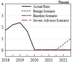
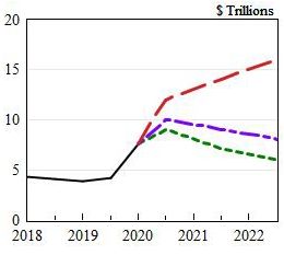
Figure 3: The Evolution of Monetary Policy under Alternative Scenarios
Target Federal Funds Rate Federal Reserve Balance Sheet
Source: Federal Reserve Board, authors’ calculations.
3.3 Severe Adverse Scenario
In this scenario, no effective vaccine or cure becomes available within the next two years, and
the threat of infection does not abate. Consequently, the recovery of economic activity and
employment is thwarted, triggering the onset of an adverse feedback loop between the real
economy and the financial system that leaves the economy mired in conditions that echo the
Great Depression of the 1930s.
With continuing high unemployment, consumer spending and business sentiment wane further.
Persistently lower household income and business revenue induce large numbers of personal
bankruptcies, business closures, and defaults on corporate debt obligations. Prices of core goods
and services start declining, and deflationary expectations become ingrained in the outlook of
financial market participants as well as consumers and businesses. Such deflation elevates the
real cost of the debt burden for households and businesses, weighing further on risk spreads and
credit conditions. That situation is exacerbated by adverse developments abroad, including
ongoing disruptions in global supply chains, persistently weak demand for U.S. exports, and
“risk-off” behavior triggered by foreign sovereign defaults and corporate bankruptcies.
In such circumstances, state and local government budgets become increasingly strapped as tax
receipts plummet, state Medicaid rolls and expenditures expand, and demand for public services
increases. Thus, the federal government faces pressure to serve as a continuing financial
backstop for states and municipalities as well as a broad swath of private sector firms.
The precise contours of such a scenario cannot be anticipated with any precision, but it seems
useful to illustrate its severity in terms of key macroeconomic variables. In particular, real GDP
picks up only slightly over coming quarters and remains far below its pre-pandemic level even at10 the end of 2022. The unemployment rate remains above 15 percent through the end of 2022. The huge shortfall in aggregate demand induces substantial declines in the core PCE price index, and headline PCE price index drops further due to weakening commodity prices. Expectations of mild deflation lead consumers to postpone spending, and elevated personal saving partly offsets fiscal efforts to lift aggregate demand. 4. Historical Lessons Extreme economic events like depressions, financial crises, and world wars require extreme policy actions. Pandemics like Covid-19 are associated with all three phenomena and differ significantly from garden variety cyclical fluctuations. In the face of a deep economic contraction and soaring unemployment, the Fed can learn important lessons from key historical episodes – including the Spanish flu pandemic, the onset of the Great Depression, the end of World War II, and the global financial crisis of 2007-2009—as well as the process of economic and policy normalization following each of these shocks. 4.1 The Spanish Flu Pandemic The world has seen many disastrous pandemics over recorded history. Among the very worst was the Black Death of 1331-1353, an outbreak of bacterial plague that killed between one-third and one-half of the population of Europe. The resulting shortage of labor led to a monumental change in the structure of Europe’s society and economy, including the end of feudalism and the onset of the agricultural revolution and, eventually, the industrial revolution. Although not nearly as lethal as the plague, the Spanish Flu of 1918-1919 has been the worst pandemic in modern history, causing 675,000 deaths in the United States and roughly 50 million deaths worldwide. Subsequent epidemics have been less destructive: the 1957 Asian flu, the 1968 Hong Kong flu, and more recently, SARS and Ebola. The initial outbreak of Spanish flu occurred during spring 1918 in midwestern U.S. Army camps and then spread to Europe as U.S. troops crossed the ocean to join the fight. The return of the troops to the US in the fall of 2018 generated an even more deadly second wave, with the peak incidence occurring between September and December 1918 as the pandemic spread westward across the country. As in the current pandemic, the densely populated northeast was the region most severely affected. 6 No vaccine or antiviral treatment was available at that time; indeed, virus strains were not identified as distinct from bacteria until nearly two decades later. In contrast to COVID-19 6 Ferguson (2020) compares the Asian Flu epidemic to the Spanish Flu pandemic and the COVID-19 pandemic. However, the epidemiological analysis of Viboud et al. (2016) concluded that the excess fatalities from the Asian flu (beyond the mortality that would typically occur during the flu season at that time) was about 13,000 in the United States – far lower than the impact of the current pandemic.
11

(which is most dangerous for middle-aged and older adults), the mortality rate from Spanish flu
was highest for adults ages 20 to 40 years, and the fatalities comprised roughly 0.5 percent of the
U.S. labor force at that time. 7

Nonetheless, unlike the current pandemic, the Spanish Flu did not lead to a major U.S. recession;
rather, the downturn was brief, and the economy exhibited a rapid V-shaped recovery. 8 The
NBER did record a recession over the period from August 1918 to April 1919, but the Balke-
Gordon data indicate that real GNP declined only slightly on a year-to-year basis. Industrial
production fell 20 percent from July 1918 to January 1919, followed by a very rapid rebound.
Other indicators -- including retail sales, purchases of consumer durables, and measures of
employment -- also dropped sharply during autumn 1918 and then recovered briskly. For
example, employment in New York fell 15 percent, but that decline only lasted a few months.

By contrast, the Spanish flu continued spreading across Europe and around the globe until early
1920. The U.K. economy experienced a more serious recession, while Barro and Ursua (2019)
have analyzed a large panel of countries and found a 5 percent drop in global output.

As in the current pandemic, non-pharmaceutical interventions (NPI) were instituted in most
cities, including the banning of large gatherings, closure of churches and synagogues, and
admonitions regarding facemasks and hand-washing. However, no city had a total lockdown,
so these NPIs did not directly affect manufacturers or other productive sectors of the economy.
Indeed, the recent analysis of Correia, Luck and Verner (2020) finds that NPIs were effective
in “flattening the curve” without impairing economic activity: Cities that imposed early and
forceful NPIs (such as St. Louis) had lower mortality rates relative to other cities (such as
Philadelphia) that did not adopt such measures.

In light of these patterns, why was the economic impact of the Spanish flu so mild compared to
the economic collapse induced by the COVID-19 pandemic? Several considerations are relevant:

Structural Differences. As of 1918, about half of the U.S. population lived on farms and in
small towns, and economic activity was dominated by agriculture, mining, and manufacturing.
By contrast, only one-fifth of the population lives in rural areas, and the bulk of employment
is in the retail trade and service sector, which are much more susceptible to disruption from a
pandemic.

The Context of World War I. During 1917-1918, the U.S. government’s share of economic
activity was nearly 40 percent, as factories, mines, and shipyards operated at full capacity to
meet its demands for materiel. 9 Moreover, about 3 million men (about 6 percent of the U.S. labor

7
  The fatality rate for the 20 to 40 group was approximately 1 % ( Gagnon et al 2013). Today the fatality rate is
highest for people over 50. It reaches 11% for those aged 70-79. By comparison, according to the SIR models, were
the covid -19 pandemic to go unchecked it would lead to a mortality shock similar or worse than 1918.
8
  See Bordo and Haubrich (2017) and Velde (2020).
9
  See Benmelech and Frydman (2020).
12

force ages 18 to 45) were serving in the armed forces. Consequently, wartime production and
employment likely dampened the negative economic shock, especially during the early stages
of the pandemic.

Social Norms. Just prior to WWI, life expectancy at birth was around 50 years for males and
55 years for females, and rates of infant mortality and maternal mortality were extremely high.
And the war itself was associated with massive loss of life, including 114,000 U.S. soldiers
as well as millions of Europeans (both soldiers and civilians). Moreover, the dissemination
of information was far more limited than the current context. 10 In that context, the elevated death
rate associated with the Spanish flu was seen as horrific but not cataclysmic. By contrast, life
expectancy today is roughly 50% longer (76 years for males and 81 years for females).
Many diseases that were previously associated with high fatalities are now treatable by
antibiotics or vanquished by universal vaccination. Consequently, the prospect of hundreds
of thousands or millions of fatalities from a pandemic is now viewed as far more catastrophic
compared with a century ago. 11

Mandated Lockdowns. As noted above, U.S. cities imposed some restrictions on large
gatherings in 1918, but stores were not closed and factories were not shuttered. By contrast, a
large swath of the U.S. economy has been closed by legal order over the past couple of months.
Several new studies have integrated epidemiological features into conventional macroeconomic
models; those model simulations suggest that the pandemic would cause a significant downturn
and job losses even in the absence of any legal restrictions but conclude that the mandated
lockdowns may account for a substantial fraction of the recent decline in U.S. economic
activity. 12 Nonetheless, the economy may not rebound fully even after those legal restrictions are
lifted, especially if middle-aged and older adults remain cautious about the hazards of resuming
their previous behavioral patterns.

4.2 The Great Depression

The Great Contraction of 1929-33 was the most severe U.S. economic downturn of the last
century. It was likely precipitated because of policy failures in the US and elsewhere. The initial
downturn in 1929 was triggered by the Federal Reserve’s adherence to the flawed “real bills”
doctrine as well as failures of corporate governance. 13 The Fed’s subsequent failure to act
as a lender of last resort resulted in a series of disastrous banking panics starting in 1930.

10
   Local newspapers played the role now occupied by social media, and the wire services were quite efficient in
disseminating information. However, the Sedition Act of 1918 imposed a broad prohibition on any ‘disloyal’
communications that could undermine the war effort, and violations of that Act were subject to imprisonment for
up to 25 years. Indeed, the term Spanish flu apparently reflects the fact that Spain was a neutral power that did not
censor the press, and hence it became the first location where the outbreak of the pandemic was widely publicized.
11
   See Ferguson (2020).
12
   See Atkeson (2020), Eichenbaum, Rebelo and Trabant (2020), and Jones and Villaverde (2020).
13
   See Meltzer (2002) and Bordo and Prescott (2019).
13

Consequently, a moderate recession turned into a severe and protracted depression. 14 The
unemployment rate rose above 25 percent, while real economic activity and aggregate prices
fell more than 30 percent. Subsequent analysis has shown that the negative monetary shock
was propagated to the real economy via rigid nominal wages. 15 Other propagation mechanisms
included debt deflation, the financial accelerator, and rising real interest rates. 16 In the global
economy, adherence to the gold standard both transmitted shocks between countries and also
prevented mitigation by monetary and fiscal policy actions. 17

The Great Contraction ended in March 1933 with actions undertaken by the incoming President,
Franklin D. Roosevelt. The first was a banking holiday in early March when all the nation’s
commercial banks were closed for a week and then only sound banks were allowed to reopen.
This ended the serious banking panic of 1932-33 by reassuring the public that their deposits were
safe. The second was taking the US off the gold standard in April and removing ‘golden fetters’,
that is, the constraints on expansionary monetary policy resulting from the gold standard. 18
Recovery was fueled by a 60% devaluation of the dollar in January 1934 as well as massive gold
inflows that fueled monetary expansion.

The Fed did not play an active role during this period, partly due to its continuing adherence to
the real bills doctrine. 19 The Fed was granted enormous new powers in the 1935 Banking Act
but did not use them. It was subsequently subordinated to the U.S. Treasury to keep interest rates
low to facilitate the fiscal actions of the New Deal. There is considerable debate over whether
those fiscal policies were key determinants of the recovery. 20 Regardless, the global slump only
fully ended with the rearmament leading to World War II.

The analogy of the Great Depression is highly relevant to understanding today’s economic
meltdown because of its depth and breadth and the propagation mechanisms and interactions
between the financial system and the economy and the failure of the Fed to act. The collapse of
aggregate demand, consumption, investment, labor markets, business failures, deflation, debt
default, and collapse of the non-bank financial sector, involved at its most acute stage a decline
of real GDP exceeding 10 percent. The collapse induced by the COVID-19 pandemic seems like
the Great Depression on steroids; real GDP is projected to fall more than 10 percent (non-
annualized rate) from March through June 2020.

14
   See Friedman and Schwartz (1963).
15
   See Bordo, Erceg, and Evans (2000).
16
   See Fisher (1933), Bernanke (1983), and Hamilton (1992).
17
   See Friedman and Schwartz (1963) and Eichengreen (1992).
18
   See Eichengreen (1992).
19
   See Meltzer (2003).
20
   See Romer (1992), Cole and Ohanian (2004), Eggertson (2008), and Jacobson, Leeper, and Preston (2016).
14

4.3 The End of WWII

Government leaders and many others view the current U.S. government’s efforts to stem the
Covid-19 pandemic as equivalent to the total mobilization of resources during World War I and
World War II. In both cases, the enemy was viewed as an existential threat, and all the country’s
resources were dedicated towards achieving victory. The U.S. involvement in World War I was
short-lived but many of the policies adopted then were perfected on a much larger scale in
World War II. 21

During the war, resources of labor, goods, and production capacity were diverted from private
peacetime uses to the government’s military uses – a tradeoff that economists often characterize
as “guns vs. butter.” More than 16 million people (including conscripted individuals as well as
volunteers), of whom 400,000 died in battle. Private-sector factories were mandated to transform
from producing peacetime goods to war materiel, accomplished by a mix of direct regulations,
rationing of goods and services, imposition of credit controls, and appeals to patriotism. 22

The total cost of World War II represented about 175 percent of GDP as of 1945. 23 This massive
increase in government expenditures was financed by a combination of taxes, bond issuance, and
elevated inflation (commonly known as the “inflation tax”). 24 The ratio of gross debt to GDP
rose from about 40 percent in 1939 to around 120 percent in 1945. 25 Following the end of the
war, the gross debt declined steadily to a trough of about 35 percent of GDP in 1974, mainly
due to a combination of rapid economic growth, mild inflation, and persistent primary surpluses.

This wartime fiscal expansion was accommodated by the Federal Reserve, which deferred to the
Treasury Department in alleviating the costs of debt issuance by implementing low interest rate
pegs (3/8 percent on short-term Treasuries and 2½ percent on longer-term Treasuries). The
inflationary consequences of this monetary policy were partially mitigated by wage and price
controls; thus, wholesale prices rose at an annual rate of 4.5 percent from 1941 to 1945.

At the end of the war, policymakers feared a renewal of the deflation and depression of the
1930s, or even a more mild downturn similar to the aftermath of World War I. They ignored the
burst of consumer spending and the surge in business investment that occurred once hostilities
ceased and rationing ended. The accommodative low interest rate peg policy was continued, and
once price controls were removed, inflation accelerated: Wholesale prices rose at an average
annual pace of 15 percent from 1945 to 1948. Consequently, Chairman McCabe and other Fed

21
   See Rockoff (2015).
22
   See Higgs (2006).
23
   The cost was $307 billion in current dollars and would be equivalent to nearly $5 trillion now; see White (2020).
24
   Taxes covered 42 percent of the total cost, while the remainder was covered by bond issuance (34 percent) and the
inflation tax (24 percent); see Friedman and Schwartz (1963).
25
   See Hall and Sargent (2020). Following the end of the war, the gross debt ratio was reduced to 35 percent, mainly
via rapid economic growth combined with persistent primary surpluses; see Cochrane (2020).
15

officials expressed growing concern over high and variable inflation, leading to rising tensions
between the Federal Reserve and the Treasury. 26

As the exigencies of the war began to fade and inflation pressures mounted, Fed officials started
a campaign to free the Fed from the dominance of the Treasury and restore its independence,
eliminating the interest rate peg and allowing the Fed to tighten monetary policy as needed to
restore price stability. This outcome was finally achieved in the Federal Reserve - Treasury
Accord of February 1951.

A key lesson from World War II is that once the pandemic passes, high inflation may be
generated if the Fed does not unwind its emergency expansionary monetary policies. 27 A similar
lesson of over -extended monetary policy is provided by the second half of the 1960s, when the
Fed kept interest rates too low to accommodate fiscal deficits resulting from domestic programs
(The Great Society) and the intensification of the Vietnam War. Those actions ushered in a
decade of high inflation that was finally ended by the Volcker Fed in 1980-82.

4.4 The Global Financial Crisis

Over the past decade, a huge number of studies have analyzed various aspects of the global
financial crisis (GFC). Here we focus on four specific issues that seem particularly relevant
under present circumstances: (1) the failure to identify the emerging risk of a financial crisis;
(2) the absence of a clear strategy for serving as lender of last resort; (3) the ineffectiveness of
the Fed’s measures for providing additional monetary stimulus at the zero lower bound (ZLB);
and (4) the sequence of major revisions to the Fed’s exit strategy and the longer-term
consequences for the size and composition of its balance sheet.

Risk Analysis. In contrast to the COVID-19 pandemic, the onset of the GFC was not a sudden or
unforeseeable event. Indeed, as Shiller (2008) noted in an incisive commentary, numerous
warnings were raised well in advance but were largely ignored by policymakers at the Fed and
elsewhere. 28 At a high-profile Fed conference, Rajan (2005) flagged the dangers of growing
financial imbalances but was harshly criticized by other attendees. Unfortunately, such reactions
were symptomatic of excessive insularity, complacency, and groupthink. 29

During the early stages of the GFC, from autumn 2007 through early spring 2008, the FOMC
reduced its federal funds rate target by a cumulative total of 3 percentage points. Some analysts

26
   See Meltzer (2003).
27
   Another risk is that the run-up in the debt to GDP ratio which may match or exceed the World War II level may
not be reduced as readily as after the war.
28
   For example, in the second edition of his book on irrational exuberance, Shiller (2005) clearly stated that a
catastrophic collapse of the housing boom could induce a worldwide recession, while Lewis (2010) highlights the
financial market participants who succeeded in trading on that risk. Taylor (2007), Bordo and Landon-Lane (2013)
and others have concluded that the Fed’s monetary policy exacerbated the housing boom that precipitated the GFC.
29
   See Archer and Levin (2018).
16
Figure 4: The Federal Reserve Staff’s Assessment of Risks
to the Economic Outlook as of September 10, 2008
Greenbook Outlook Actual Unemployment
Note: The 70 percent and 95 percent confidence intervals generated by the FRB/US model
are denoted by the dark and light shaded areas, respectively.
have concluded that the stance of monetary policy was still too tight. 30 Nonetheless, at its
meetings in June and August, the FOMC decided to stand pat in light of its concerns about
upside risks to inflation. The next FOMC meeting was held on September 16, 2008—just
one day after the failure of Lehman Brothers, the fourth largest U.S. investment bank and key
counterparty to a huge array of outstanding financial transactions. At that juncture, one might
reasonably have expected the FOMC to take decisive action while issuing a sober but reassuring
press release. But in fact, the FOMC took no action and merely stated that “the downside risks
to growth and the upside risks to inflation are both of significant concern to the Committee.”
Indeed, that outcome reflected a unanimous FOMC decision, i.e., ten ayes and no dissents.
The views of FOMC members at that September 2008 meeting were broadly in line with the
background analysis provided by Federal Reserve Board staff. The staff outlook (which was
called the “Greenbook”) had been circulated a few days earlier, so the chief domestic economist
provided an update at the FOMC meeting indicating that “...we’re still expecting a very gradual
pickup in GDP growth over the next year and a little more rapid pickup in 2010.” 31 Further
30
See Hetzel (2012) and Bordo (2014).
31
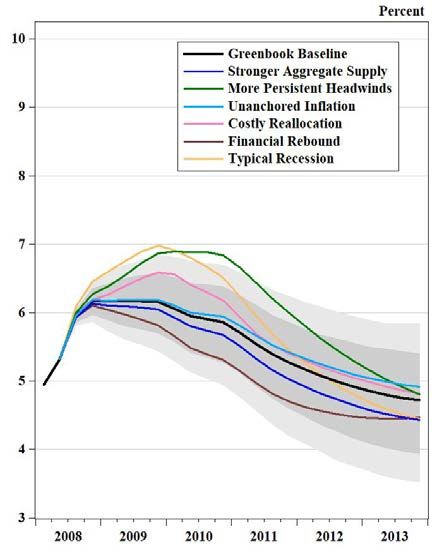
See FOMC Meeting Transcript, September 16, 2008, p.20.17 insight into the staff outlook can be garnered from the Greenbook itself, which was subsequently released to the public after a five-year lag. In particular, the left panel of Figure 1 reproduces the staff’s assessment of risks to the outlook for unemployment as presented in its September 2008 Greenbook. The shaded areas denote confidence intervals for the benchmark forecast (the “fan chart”), which indicated odds of 50:1 that the unemployment rate would remain below 7 percent. 32 The alternative scenarios were intended to characterize a range of macroeconomic outcomes that would be broadly consistent with the model-based confidence intervals; these sources of risk included benign developments (such as a financial rebound) as well as adverse developments (such as persistent headwinds or a typical recession). By contrast, the right panel shows the actual evolution of the unemployment rate following the collapse of Lehman and the intensification of the GFC. Evidently, the Fed staff’s analysis was severely deficient in gauging the true magnitude of risks to the U.S. economic outlook, even as the financial system was teetering on the edge of collapse. This episode underscores one of our key recommendations in section 2 above, namely, the Federal Reserve needs to foster and sustain a work environment that encourages openness and outside-the-box thinking, so that Fed officials can clearly identify material risks to the economy and formulate plans for mitigating those risks. Lender of Last Resort. Well before the onset of the GFC, observers regularly pointed out the Federal Reserve’s lack of any clear and systematic strategy for serving as lender of last resort (LOLR) in a financial crisis, but unfortunately those warnings were not heeded. 33 One consequence was that the Fed’s actions during the GFC were widely seen as discretionary, opaque, and unfair instead of being viewed as transparent and even-handed. Controversy has swirled ever since then about why the Federal Reserve decided to rescue one investment bank (Bear Stearns) but not another (Lehman), and why it suddenly changed course thereafter to lend funds to two other investment banks (Goldman Sachs and Morgan Stanley). 34 Similarly, the Fed’s rescue of a major insurance firm (AIG) raised questions about why it wasn’t providing similar assistant to other businesses. Consequently, the Fed was commonly subjected to criticism for helping out Wall Street while neglecting Main Street. A related issue is that the Fed misdiagnosed the early stages of the GFC as reflecting a lack of liquidity rather than the risk of insolvency. 35 The underlying problem reflected the difficulty of pricing securities backed by a pool of assets, whether mortgage loans, commercial paper issues, or credit card receivables. Pricing securities based on a pool of assets is difficult because the quality of individual components of the pool varies. Unless each component is individually 32 These confidence intervals were obtained via stochastic simulations of the FRB/US model using shocks drawn from the estimated distribution of model residuals from 1987 to 2007 (the Great Moderation era). 33 See Goodfriend and King (1988), Bordo (1990), and Meltzer (2003, 2010). 34 See Ball (2016, 2018), Bernanke (2016), and Cheng and Wessel (2018). 35 See Schwartz (2008) and Taylor and Williams (2008).
18

examined and evaluated, no accurate price of the security can be determined. Consequently,
the credit market was faced with assessing the risk of failure of financial firms whose portfolios
were filled with complex derivatives whose value could no longer be ascertained. The credit
market was thus plagued by the inability to determine which firms were insolvent, and hence
lenders became increasingly unwilling to extend credit to borrowers who might not be
creditworthy.

As financial strains intensified in spring 2008 and became a full-blown crisis after the collapse of
Lehman, the Federal Reserve began intervening directly into securities markets and taking credit
risk onto its balance sheet using its authority under section 13(3) of the Federal Reserve Act.
As Goodfriend (2011) subsequently noted, such actions necessitated the picking of winners and
losers – an intrinsically political choice best left to the fiscal authorities -- and hence posed
substantial risks to the Fed’s operational independence.

Monetary Stimulus. As the GFC subsided, the U.S. economy began to stabilize and the recession
ended in mid-2009. The unemployment rate reached a peak of nearly 10 percent later that year
and only subsided slowly over subsequent years (and even that decline partly reflected
discouraged individuals dropping out of the workforce). With the federal funds rate pinned at
zero starting in December 2008, the FOMC endeavored to foster a strong recovery using two
“unconventional” tools for providing additional monetary stimulus: forward guidance about the
target federal funds rate, and quantitative easing via large-scale purchases of Treasuries and
agency mortgage-backed securities (MBS). Nonetheless, the subsequent recovery was painfully
sluggish and took nearly a decade, the slowest U.S. recovery in the historical record, which in
turn raises substantial doubts regarding the efficacy of both of those monetary policy tools. 36

Exit Strategy. In spring 2009, the Fed began unwinding some of its short-term liquidity
programs that had helped to stabilize disorderly markets, but it maintained its holdings of longer-
dated securities. However, most of the Fed’s emergency liquidity programs were not closed until
early 2010 -- well after financial strains had subsided. The Fed could have allowed those
programs to end somewhat earlier but proceeded cautiously to avoid triggering a new bout of
financial turmoil.

By contrast, the Fed’s exit strategy for its balance sheet was relatively opaque and subject to a
sequence of major reversals and revisions. Consequently, the actual evolution of the Fed’s
balance sheet was highly discretionary and unpredictable. As evident from the “taper tantrum”
of 2013, that uncertainty contributed to elevated financial market volatility that likely hampered
the effectiveness of the FOMC’s monetary policy. 37

36
     See Bordo and Haubrich (2017), Bordo and Levin (2019), Levin (2020), and Levin and Sinha (2020).
37
     See Bordo and Levin (2019).
19 Reinvestment Policy. In mid-2009, Fed officials indicated that large reserve balances could be reduced automatically due to ongoing principal repayments on its securities holdings. 38 At its August 2010 meeting, however, the FOMC decided to prevent such shrinkage by reinvesting all principal repayments into new securities purchases. The FOMC subsequently agreed (in a near-unanimous decision in June 2011) that such reinvestments would be halted at the start of its policy normalization process, prior to implementing any increases in the target federal funds rate. In September 2014, however, the FOMC overturned that decision in a revised exit strategy that delinked the start of interest rate hikes from the onset of balance sheet normalization, and consistent with those revised principles, the reinvestment of principal repayments continued until autumn 2017 -- nearly two years after the liftoff of the target federal funds rate from the ZLB. Sales of MBS. In June 2011, the FOMC reached a near-unanimous decision that sales of its MBS holdings would commence following the first increase in the target federal funds rate and that such holdings would be eliminated over a period of three to five years. 39 However, the FOMC completely reversed that decision in its 2014 exit strategy, which stated that MBS sales were no longer anticipated; and, in fact, no such sales ever took place. Indeed, the lack of transparency about the Fed’s exit strategy continues to this day: The Federal Reserve Board has a public webpage entitled“History of the FOMC’s Policy Normalization Discussions and Communications” that makes no reference to the June 2011 exit principles, as though that nearly-unanimous FOMC decision had never been made at all. 40 5. Current Policy Challenges Guided by lessons from past crises, the Federal Reserve must now formulate a systematic and transparent approach to its lender-of-last-resort programs and its monetary policy strategy. In this context, scenario analysis and contingency planning will be crucial for sustaining public confidence, fostering the goals of maximum employment and price stability, and ensuring that the Federal Reserve retains its operational independence and credibility. In particular, effective coordination and communication with the Congress and the Treasury will be crucial. For example, the extension or unwinding of many of the Fed’s emergency programs – including the Fed’s direct business lending initiative and its purchases of municipal debt and corporate securities -- will hinge on the approval of the Secretary of the Treasury, and those plans should be ironed out well in advance. Moreover, at some stage the Federal Reserve should engage in a swap with the U.S. Treasury, exchanging its holdings of corporate bond securities for an equal amount of Treasury securities. 38 See Bernanke (2009). 39 See https://www.federalreserve.gov/monetarypolicy/fomcminutes20110622.htm. 40 See https://www.federalreserve.gov/monetarypolicy/policy-normalization-discussions-communications- history.htm.
20

Such a swap would be very helpful for normalizing the Fed’s balance sheet and sustaining its
operational independence.

5.1 Lender-of-Last-Resort Programs

In his recent testimony to the U.S. House Financial Services Committee and the U.S. Senate
Budget Committee on May 18-19, Fed Chairman Powell stated: “The tools that the Federal
Reserve is using under its 13(3) authority are for times of emergency, such as the ones we have
been living through. When economic and financial conditions improve, we will put these tools
back in the toolbox.”

Some of these emergency programs are parallel to actions taken by the Federal Reserve at the
height of the global financial crisis, including: providing short-term liquidity to primary dealers,
commercial paper, and money market mutual funds; establishing a Term Asset-Backed Loan
Facility (TALF) that purchases asset-backed securities; and extending U.S. dollar swap lines to
an expanded list of global central banks. 41 In addition, the Federal Reserve has broken new
ground in using its 13(3) authority to engage in purchases of municipal debt securities, corporate
bonds (investment-rated and certain sub-investment-rated categories) in both the primary and
secondary markets, and direct lending to businesses via the Main Street Lending Program.
(Tables A1 and A2 provide further details about those emergency actions.)

The Fed should specify the conditions under which each program will be ended or tapered. This
involves weighing the objectives and benefits of each program against their costs and risks under
the different scenarios. The Fed must also develop a strategy for communicating how and under
what conditions the individual programs should be unwound, and the expected sequencing. In
order to avoid unnecessary jarring impacts on finanical markets, clear communications will be
particularly important for the programs involving purchases of corporate and municipal debt
securities. Moreover, the Fed should specifically flag critical issues that will require
coordination with the U.S. Treasury and the Congress, and begin conducting the legwork
necessary to achieve its strategic goals.

Short-Term Liquidity Programs. In both the baseline and benign scenarios, in which the
economy recovers substantially while inflation remains subdued and financial markets quickly
regain normal operations, the Fed should prepare to quickly unwind its emergency short-run
liquidity provisions, including its Primary Dealer Credit Facility (PDFC), Commercial Paper
Funding Facility (CPFF) and its Money Market Mutual Fund Facility (MMMF). The experience
of the GFC shows that as extreme risk aversion dissipates and financial institutions resume
normal operations, the Fed’s short-term funding facilities will no longer be needed and can be
unwound promptly.

41
  The Federal Reserve has also expanded the size and scope of its repurchase agreements in the domestic market
and with other central banks.
You can also read