Keeping up with the e-Joneses: do online social networks raise social comparisons?
←
→
Page content transcription
If your browser does not render page correctly, please read the page content below
Discussion Paper
No. 2018-43 | May 25, 2018 | http://www.economics-ejournal.org/economics/discussionpapers/2018-43

Keeping up with the e-Joneses: do online social
networks raise social comparisons?
Fabio Sabatini and Francesco Sarracino

Abstract
Online social networks, such as Facebook, amplify the occasions for social comparisons
which are detrimental to well-being. The authors test the hypothesis that the use of social
networking sites (SNS) increases social comparisons using Italian data from the
Multipurpose Household Survey, and European data from Eurobarometer. The results
suggest that SNS users have a higher probability to compare their achievements with
those of others. This evidence is robust to endogeneity concerns. The authors conclude
that, by increasing the opportunities for social comparisons, SNS can be an engine of
income dissatisfaction for their users.

JEL      D83; I31; O33; Z1; Z13

Keywords Social networks; social networking sites; social comparisons; satisfaction with
income; relative deprivation

Authors
Fabio Sabatini, Sapienza University of Rome
Francesco Sarracino, STATEC (Institut National de la Statistique et des Etudes
Economiques), Luxembourg, and National Research University Higher School of
Economics; f.sarracino@gmail.com

Citation Fabio Sabatini and Francesco Sarracino (2018). Keeping up with the e-
Joneses: do online social networks raise social comparisons? Economics Discussion Papers,
No 2018-43, Kiel Institute for the World Economy. http://www.economics-
ejournal.org/economics/discussionpapers/2018-43

Received March 1, 2018 Accepted as Economics Discussion Paper May, 11, 2018 Published May 25, 2018
© Author(s) 2018. Licensed under the Creative Commons License - Attribution 4.0 International (CC BY 4.0)

1    Introduction
An old way of saying states: “The neighbour’s grass is always greener”. People
have the tendency to track their progress and assess their self-worth by com-
paring themselves to others. As a result, individuals’ satisfaction depends, at
least in part, on others’ possessions and achievements.
    The action of comparing oneself with others in order to evaluate or to en-
hance some aspects of the self is known as “social comparison”. Such behaviour
affects a variety of economic choices including consumption, investments in hu-
man capital, effort in the workplace, risk taking, and contribution to the pro-
vision of public goods just to name a few (Linde and Sonnemans, 2012; Cohn
et al., 2014; Gamba et al., 2014). In addition, social comparisons are a relevant
correlate of life satisfaction (Clark and Oswald, 1996; Ferrer-i Carbonell, 2005;
D’Ambrosio and Frick, 2007; Guillen-Royo and Kasser, 2015).
    The possibility to compare oneself with others relies on the availability of
information about the lives of others or, in other terms, on the visibility of
alternative lifestyles. Frijters and Leigh (2008) explained that leisure aspirations
depend on the visibility of the lifestyles of others, which in turn is positively
associated with the frequency and repetition of social interactions. In their
work on inequality and conspicuous leisure Huang and Shi (2015) argue that
the social comparisons that prompt emulation are likely to be linked to “the
relative visibility of consumption and leisure, the cost of display, and the social
preference in an economy.” (Huang and Shi, 2015, p. 950).
    Early studies on social comparisons have found that, on average, people re-
port comparing themselves to others about once per day (Wheeler and Miyake,
1992). There are several reasons to believe that this average may have in-
creased with the increasing penetration of SNS, such as Facebook, into users’
daily life. First, users are likely to experience an extension of their reference
group. Most users have online “friends” who are actually past friends or distant
acquaintances, whose information would not be as readily, if at all, accessible
without online social networks. Several studies, in fact, have provided evidence
that SNS allows the crystallization of weak or latent ties that might otherwise
remain ephemeral (see for example Ellison et al., 2007; Antoci et al., 2015).
Moreover, because most SNS users allow all “friends” unrestricted viewing of
their profiles (Pempek et al., 2009), individuals often have access to a large
amount of information even about their most distant acquaintances. The easy
access to such information may extend the possibilities for social comparisons.
    Second, SNS allow a more efficient access to information about “friends”
compared to offline interactions. While individuals may not meet or engage in
face-to-face conversations with close friends on a daily basis, SNS allow users
to keep in touch with, and monitor the activities of, numerous friends multiple
times a day, even when those friends are very distant.
    Most importantly, online social networks not only offer more frequent op-
portunities for comparison, but they also offer more opportunities for upward
comparisons, i.e. towards those who look better off. This is due, in particular,
to the mainly positive nature of information that people choose to display on-

                                         2
line. Psychological studies have shown that Facebook, a prominent example of
SNS, tends to serve as an onslaught of idealized existences – babies, engagement
rings, graduations, new jobs, consumption of expensive goods and services such
as cars and vacations – that invites upward social comparisons at a rate that
can make “real life” feel like just a grey routine. This evidence is supported by
studies finding that a more intense use of Facebook makes users more likely to
believe that others are “happier” and “had better lives” than people who used
the online social network less frequently (Chou and Edge, 2012). This evidence
suggests that Facebook does leave users with a positively skewed view of how
others are doing, which can be a source of frustration and dissatisfaction with
own life.
We contribute to this literature testing the hypothesis that the use of social
networking sites (SNS), such as Facebook, raises people’s tendency to compare
themselves to others in nationally representative samples. Our argument is that
online social networks disclose an unprecedented volume of personal information
that can be a powerful source of social comparisons.
Our contribution bridges two literatures. Some economic studies have anal-
ysed the ability of mass media to provide information about alternative lifestyles
and, therefore, to stimulate social comparisons that may possibly undermine life
satisfaction (Stutzer, 2004; D’Ambrosio and Frick, 2007; Guillen-Royo, 2017).
For instance, Bruni and Stanca (2006) and Hyll and Schneider (2013) anal-
ysed the role of television. Clark and Senik (2010) were the first to address
the role of Internet access in a broader study about the intensity and direction
of income comparisons. Lohmann (2015) systematically explored the effect of
information and telecommunication technologies (ICT) with a specific focus on
Internet access. We contribute to these works by studying the role of online
social networks. The second literature encompasses cross-disciplinary studies
investigating the relationship between Facebook use and happiness (Arampatzi
et al., 2016; Lim and Yang, 2015; Tandoc et al., 2015).
Our analysis uses two datasets that provide individual level information
about the use of SNS, the Multipurpose Household Survey (MHS) provided by
the Italian National Institute of Statistics (Istat), and the Eurobarometer pro-
vided by the European Commission. The 2010, 2011, and 2012 waves of the
MHS allow to explore the association between the use of online social networks
and social comparisons using a large and nationally representative number of
observations. An important advantage of this dataset is that it allows to control
for potential endogeneity using a conventional instrumental variable approach:
we exploit the availability of fast Internet access across Italian regions as a
source of exogenous variation. Territorial differences in broadband coverage
depend on orographic features that exogenously determined the technological
characteristics of the old voice telecommunication infrastructures. In section 3
we illustrate how, several decades after their construction, these infrastructures
unpredictably turned out to be broadband-friendly or not depending on their
early characteristics, thereby forming the basis for a natural quasi-experiment
in the availability of fast Internet. In addition, we account for possible reverse
causality using generated instrumental variables (Lewbel, 2012). This method
3consists in generating instrumental variables (IV) from existing data to run
two-stages least squares (2SLS) regressions when the exclusion restrictions for
conventional IV are weak or do not hold. To test the generality of our find-
ings from Italy, we turn to Eurobarometer data, which provides cross-country
and nationally representative information about people’s use of SNS and their
propensity to compare to others. The downside of using Eurobarometer data is
that we lack instruments to account for possible endogeneity. To address this
issue, we follow Lewbel’s identification strategy (Lewbel, 2012). We use the
2011, 2012, and 2013 waves for comparability with the results from Italy.
Our results suggest that SNS users have a higher probability to compare
their achievements with those of others. This effect seems stronger than the
one exerted by TV watching, it is particularly strong for younger people, and it
affects men and women in a similar way.
The paper begins by providing the motivation of the study and briefly review-
ing the related literature (Section 2). We then describe our data and empirical
strategy in Section 3. In Section 4 we present and discuss our results. Section
5 concludes.
2 Related literature
In economics, the study of the satisfaction and dissatisfaction driven by social
comparisons can be traced back to the very origins of the concept of utility.
As Bentham (1781) used it, utility refers to pleasure and pain, the “sovereign
masters” that “point out what we ought to do, as well as determine what we shall
do” (Kahneman et al., 1997). Bentham explained how the pleasures and pains
enjoyed and suffered by others are fundamental sources of human satisfaction
and dissatisfaction. “The pleasures of malevolence are the pleasures resulting
from the view of any pain supposed to be suffered by the beings who may
become the objects of malevolence”. “The pains of malevolence are the pains
resulting from the view of any pleasures supposed to be enjoyed by any beings
who happen to be the objects of a man’s displeasure” (Bentham, 1781, pp.
37-40).
Marx explained the relative nature of utility in his early work on wage,
labour, and capital: “Our wants and pleasures have their origin in society;
we therefore measure them in relation to society; we do not measure them in
relation to the objects which serve for their gratification. Since they are of a
social nature, they are of a relative nature” (Marx, 1847, p. 45). Nearly fifty
years later, Veblen (1899) introduced the concept of ‘conspicuous consumption’,
serving to impress other persons.
However, the term social comparison was introduced by Festinger (1954) in
a paper in which the author explained the role of social comparisons in eval-
uating own opinions and abilities: “To the extent that objective, non-social,
means are not available, people evaluate their opinions and abilities by compar-
ison respectively with the opinions and abilities of others” (p. 118). Festinger
also implicitly introduced the concepts of downward and upward comparisons
4(which were later formalized by Wills (1981)) by arguing that “The tendency
to compare oneself with other specific person decreases as the difference be-
tween his ability or opinions and one’s own increases” (p. 120). For example,
an undergraduate student in an average college does neither compare herself
to inmates of an institution for feeble minded (which would be a “downward
comparison”), nor to colleagues attending a PhD program in a top university
(“upward comparison”). In fact, comparisons with so distant others would nec-
essarily be inaccurate.
Yet, it was Duesenberry (1949) the first one to empirically test the impor-
tance of relative income for utility. His results suggested that upward compar-
isons overcome downward comparisons in determining people’s aspirations and
satisfaction. Aspirations, in fact, tend to be above the level already reached. As
a result, wealthier people impose a negative externality on poorer people, but
not vice versa.
Wheeler and Miyake (1992) explained that comparisons about performance
(also called “similar comparisons”) are more frequent between close friends.
Upward and downward comparisons (also called “dissimilar comparisons”), on
the other hand, are more frequent in more distant relationships. This kind of
comparison is more likely to occur in online social networks than in face-to-
face interactions, since SNS like Facebook allow users to interact with – or to
silently observe the lifestyles of – distant others such as friends of friends, distant
acquaintances or public figures.
Brickman and Bulman (1977) suggested that close friends generally want
to avoid upward and downward comparisons because they are concerned with
the negative feelings that they might prompt. This may result in a particular
delicacy in reporting about specific life events or achievements in face-to-face
conversations with friends. For example, a happily married individual may want
to use tact in talking about her marriage to a friend who has just divorced.
SNS-mediated interactions, on the other hand, usually start with the unilateral
sharing of information with an indistinct audience (Arampatzi et al., 2016). In
this context, individuals are less likely to be concerned with specific friends’
feelings. The simplified forms of communication offered by SNS – such as the
acts of posting a “status” or sharing a photo – offer less ways to adopt delicacy
and tact in dealing with others. In addition, Facebook research has proved that
most users tend to over-share the bright side of their lives – e.g. consumption
of vacations, culture, or expensive goods and services – to impress others and
to attain or maintain a given social status.
Even if face-to-face interaction provides many opportunities to witness the
conspicuous consumption of friends, SNS-mediated interaction offers more chances
to acquire detailed information about friends’, acquaintances’, as well as distant
or unknown others’ lifestyles. For SNS users, it is virtually impossible to avoid
seeing such information because of the very nature of the news feed, in which
“friends” post their “status” on a regular basis.
The empirical literature has operationalized the concept of social compar-
isons through measures of income aspirations, relative deprivation, and dissat-
isfaction with income. The first tests of the role of social comparisons suggested
5that individuals’ income aspirations are influenced by face-to-face interactions.
Using a cross-section of Swiss survey data, Stutzer (2004) showed that a higher
income level in the community determines higher individual aspiration levels,
and that the discrepancy between income and aspiration matters for well-being.
The more an individual interacts with her neighbours, the more the income
situation of the community where she lives matters in defining her aspirations.
Bruni and Stanca (2006) used World Values Survey (WVS) data to analyse
the effect of television, an agent of consumption socialization, on income aspi-
rations. Their results indicate that the effect of income on subjective well-being
is significantly lower for heavy-TV viewers. Bruni and Stanca explain that “by
watching TV people are overwhelmed by images of people richer and wealthier
than they are. This contributes to shifting up the benchmark for people’s posi-
tional concerns: income and consumption levels are compared not only to those
of their actual social reference group, but also to those of their virtual reference
group, defined and constructed by television programs. As a consequence, tele-
vision viewing makes people less satisfied with their income and wealth levels”
(2006, p. 213).
If television, a unidirectional mass medium that provides relatively limited
information about the lives of others, affects income aspirations and viewers’
satisfaction with their income, it seems reasonable that online social networks,
which allow interactive communication and provide an unprecedented volume
of personal information, can affect income aspirations even more.
Surprisingly, the role of social media has received little attention in eco-
nomics. Based on data drawn from the third wave of the European Social
Survey, Clark and Senik (2010) found that individuals with Internet access tend
to attach greater importance to income comparisons. Using panel data from
the European Union Statistics on Income and Living Conditions (EU-SILC),
Lohmann (2015) found that stated material aspirations are significantly pos-
itively related to fast-Internet access. Lohmann also reported cross-sectional
evidence from the WVS suggesting that people who regularly use the Internet
as a source of information derive less satisfaction from their income. Due to
lack of data, these authors could not assess how material aspirations relate to
the use of online social networks.
A few psychological studies have assessed the possible effects of Facebook on
users’ self-esteem, feelings of deprivation, and subjective well-being. Based on
an online survey of 736 college students recruited via email from a large Mid-
western university, Tandoc et al. (2015) found that the use of Facebook triggers
feelings of envy, which expose users to the risk of depression. Lim and Yang
(2015) used the survey responses of 446 university students attending a Korean
university to study the emotional effect of social comparisons occurring in a
SNS environment. Their results suggest that a predominant activity in SNS is
making social comparisons with public figures and that such comparisons trigger
a range of emotional responses including envy and shame. Based on a survey
administered to 231 young adults recruited by two students at the University
of Amsterdam through their online social networks, de Vries and Kühne (2015)
found that Facebook use was related to a greater degree of negative social com-
6parison, which was in turn related negatively to self-perceived social competence
and physical attractiveness. The main limitation of this body of research resides
in the use of small, and biased samples, in most cases composed of self-selected
groups of undergraduate students attending specific colleges. We assess the re-
lationship between SNS use and social comparisons in large and representative
samples.
3 Data and empirical strategy
The empirical analysis uses two individual level datasets providing information
on the use of online social networks. First, we investigate the relationship be-
tween SNS use and proxies of social comparisons using the 2010, 2011 and 2012
waves of the MHS provided by Istat. Second, we use the 2011, 2012 and 2013
waves of the Eurobarometer survey provided by the Public Opinion Analysis
sector of the European Commission.
The two datasets provide similar information about individuals’ use of SNS
along with their personal characteristics, perceptions, and behaviors. The Ital-
ian dataset, however, allows to exploit the availability of broadband across re-
gions as a potential source of exogenous variation to implement a standard IV
estimation strategy. Moreover, the MHS contains valuable information about
how people connect to the Internet that is, unfortunately, not available in the
Eurobarometer. The latter, on the other hand, allows to tackle the issue of
social comparisons extending the analysis to 18 European countries.1
The use of two different surveys allows to test the robustness of our find-
ings and to check the causal relationship among variables using two estimation
strategies: in the case of Eurobarometer we use 2SLS with generated instruments
(Lewbel, 2012); in the case of the Italian MHS we use 2SLS with standard in-
strumental variables, and with generated instruments. This allows also to check
the consistency of Lewbel’s method by comparing its results with those from
standard instruments applied to the same dataset.
In both datasets we use people’s dissatisfaction with their financial situation
to measure social comparisons. Financial dissatisfaction is strongly correlated
with relative deprivation (D’Ambrosio and Frick, 2007, 2012) and several studies
used financial dissatisfaction as a proxy of social comparisons (see for example
Brockmann et al., 2009; Bartolini and Sarracino, 2015). Moreover, seminal work
in psychology theorized that dissatisfaction is tightly linked to social compar-
isons. For example, in their pioneering study on the attitudes of American
soldiers during World War II, Stouffer et al. (1949) found that soldiers’ feelings
of dissatisfaction with their own condition were less related to the actual degree
of hardship they experienced than to the situation of the unit or group to which
they compared themselves. In other words, dissatisfaction basically depends
on social comparisons. More recently, economic studies have ascertained that
1 The countries included in the analysis are: Austria, Belgium, Cyprus, Denmark, Finland,
France, Germany, Greece, Ireland, Italy, Luxembourg, Malta, Netherlands, Portugal, Spain,
Sweden, Turkey, United Kingdom.
7satisfaction with own financial situation and subjective well-being are driven
by the gap between the individual’s income and the incomes of all individuals
richer than him/her (Clark and Oswald, 1996; Bossert and D’Ambrosio, 2006).
More specifically, using panel data, D’Ambrosio and Frick (2007, 2012) show
that financial dissatisfaction is strongly associated to a measure of relative de-
privation, while it weakly correlates with absolute income. That is to say that
financial dissatisfaction mirrors relative rather than absolute standards, thus
reflecting social comparisons, i.e. individual achievements with respect to what
other people – with whom the respondent compares herself – get. Additionally,
the inclusion of a control for absolute income allows to control for its possible
confounding effects on financial dissatisfaction, thus allowing the latter to proxy
relative concerns.
In the MHS, financial dissatisfaction is measured through responses to the
question: “How satisfied do you feel with your financial conditions?”, where
possible responses were “very satisfied”, “fairly satisfied”, “not much satisfied”
and “not at all satisfied”. The scale of the answers has been reverted so that
higher scores stand for more dissatisfaction. The use of SNS is measured through
a binary variable capturing respondents’ use of online social networks such as
Facebook and Twitter.
In the Eurobarometer, financial dissatisfaction is observed through answers
to the question: “How would you judge the current financial situation of your
household”. The answers range on a scale from 1 (‘very good’) to 4 (‘very
bad’). The use of SNS is measured through the answers to the question: “To
what extent do you use online social networks?”. The answers range on a scale
from 1 (‘everyday’) to 6 (‘never’).
Since financial dissatisfaction, our dependent variable, is ordered in 4 cat-
egories – in both datasets – we adopt an ordered probit model. Formally, our
baseline equation is as follows:
1 if 0 < yi ≤ c1 ,
2 if c < y ≤ c ,
1 i 2
financial dissatisfactioni = (1)
3 if c 2 < y i ≤ c 3,
4 if c3 < yi ≤ c4 ,
where 0 < c1 < c2 < c3 < c4 ;
the index i stands for individuals;
and c1 - c4 are unknown parameters to be estimated.
Yi = α + β1 · SN Si + θ · Xi + εi , εi ∼ N (0, 1)
Yi is financial dissatisfaction, SN Si is the use of SNS, θ is a vector of parameters
for the vector of control variables Xi and εi is a vector of normally distributed
errors with mean equal to zero and standard deviation equal to one. In the
regressions on Italian data, we use robust standard errors. In case of Euro-
barometer data, we use standard errors clustered at country and year level.
8The list of control variables includes:
• Age, gender, marital status, family size, education, and work status.
• The time spent watching television. This is measured through the fre-
quency of TV watching in the Eurobarometer – on a scale from 1 (‘never’)
to 6 (‘nearly every day’), and through the number of minutes spent watch-
ing TV per day in the MHS. This control was included to account for the
role of television for material aspirations (Bruni and Stanca, 2006).
• A dummy for each year when the data were collected.
Additionally, in the MHS-based analysis we also controlled for:
• Fast Internet access, measured through the use of a broadband connection
given by DSL or optical fibre.
• The frequency of meetings with friends, to account for the possible re-
lationship of face-to-face interactions with material aspirations (Stutzer,
2004).
• Regional level controls including the real per capita GDP, and internet
penetration among families, and the share of residents with higher school
education. These variables are meant to control for heterogeneity among
regions.
The list of controls in the Eurobarometer-based analysis also includes the fol-
lowing variables:
• the real GDP per capita;
• the size of respondents’ town of residence;
• respondents’ placement in society as derived from the question: “Do you
see yourself and your household belonging to?”. Answers range on a scale
from 1 (‘The lowest level in society’) to 10 (‘The highest level in society’).
• an index of media use reflecting respondents’ exposure to media.
Descriptive statistics are reported in table 1 for the Italian sample and 2 for
Eurobarometer data.
TABLE 1 APPROXIMATELY HERE
TABLE 2 APPROXIMATELY HERE
3.1 Endogeneity issues
The coefficients from equation 1 indicate the sign and magnitude of partial
correlations among variables. However, we cannot discard the hypothesis that
the use of SNS is endogenous to financial dissatisfaction. Personal characteristics
can correlate with both the use of SNS and the dependent variable. Hence, we
turn to two-stages least squares (2SLS) to check the robustness of our findings
to possible endogeneity bias.
93.1.1 Multipurpose Household Survey
For the Italian data two different identification strategies are possible: one based
on Lewbel’s method (2012) – which we will describe in greater detail in the next
subsection – and one exploiting the availability of fast Internet access across
Italian regions as a source of exogenous variation (Sabatini and Sarracino, 2017).
In particular, we identified the two following instruments:
1. The percentage of the population for whom a DSL connection was avail-
able in respondents’ region of residence according to data provided by the
Italian Ministry of Economic Development. DSL (digital subscriber line,
originally digital subscriber loop) is a family of technologies that provides
Internet access by transmitting digital data over the copper wires of a
traditional local telephone network.
2. A measure of the digital divide given by the percentage of the region’s area
that was not covered by optical fibre, elaborated from data provided by
The Italian Observatory on Broadband. Optical fibre permits transmission
over longer distances and at higher speed than DSL.
Both variables were measured in 2008, two years before the first wave of
the Multipurpose Household Survey, which we employ in our study. The valid-
ity of the instrument is justified by the fact that the availability of broadband
basically depends on orographic features that exogenously determined the tech-
nological characteristics of the old voice telecommunication infrastructures sev-
eral decades before the advent of the Internet. In the 2000s, the old telephone
infrastructures unpredictably turned out to facilitate or to hamper the estab-
lishment of broadband depending on a specific early characteristic called ‘local
loop’. The local loop is the distance between final users’ telephone line and the
closest telecommunication exchange or ‘central office’. The longer the copper
wire, the less bandwidth is available via this wire. If the distance is above a cer-
tain threshold (approximately 4.2 kilometers), then the band of the copper wires
cannot be wide enough to support a broadband Internet connection (Campante
et al., 2013). When traditional telephone infrastructures were built, for the most
part in the 1970s, the length of copper wires was exogenously determined by the
orographic features of the territory. If there were natural or artificial obstacles
between users’ telephone lines and the central office – such as, for example, a hill
or a railroad – then the length was likely to exceed the 4.2 kilometers threshold
(Between, 2006; Ciapanna and Sabbatini, 2008).2 In the 2000s, the length of
the local loop unpredictably turned out to be a crucial factor for broadband
accessibility, forming the basis for a natural quasi-experiment in the availability
of fast Internet: Regions with relatively short local loops were advantaged in
the diffusion of the broadband and where characterized by a better broadband
coverage in the 2000s.
2 In Appendix B, we provide a map illustrating the orographic characteristics of the Italian
territory and one showing the broadband coverage in 2007. The latter suggests that, in Italy,
the most impervious territories are those with the worst broadband coverage.
10As for the second instrument, when the broadband connection cannot be
implemented through pre-existing copper wires, it is necessary to turn to an
optical fibre-based technology to provide fast-Internet. The possibility and the
costs of installing this type of infrastructure, however, even more strongly rely on
the exogenous characteristics of the natural environment. In fact, optical fibre
entails the need to install new cables underground. This involves excavation
works, which are expensive and generally delay or even prevent the provision of
broadband in the area.
The tests of over-identifying restrictions support the assumption of the or-
thogonality of the instruments.
For any given set of orographic characteristics of an area, the provision of
broadband – whether through DSL or optical fibre technology – may also have
been influenced by some socio-demographic factors that affected the expected
commercial return on the provider’s investment, such as population density,
per capita income, the median level of education and the local endowments of
social capital. These characteristics may correlate with our outcomes of interest
in ways that could confound causal interpretation. To account for possible
confounding effects, we control also for the regional level of per capita GDP,
and internet penetration among families.
We use the two instruments in a 2SLS model implemented in Stata by the
ivreg2 command. Angrist (2001) showed that the coefficients estimated with
a linear 2SLS are equal to the marginal effects produced by non linear instru-
mental variables models even in presence of discrete dependent variables. More-
over, although our endogenous variable is categorical, we adopt Ordinary Least
Squares (OLS) in the first step because only OLS estimates produce residuals
that are uncorrelated with fitted values and covariates, thus providing a valid
instrumental variable (Angrist and Pischke, 2009). The first step can be written
as:
SN Si = π1 + π2 · z1 + π3 · z2 + π4 · Xi + νi (2)
where z1 and z2 are the two above-mentioned instruments, Xi is a vector of
control variables, and νi is the error term.
The second step is as follows:
financial dissatisfactioni = α + β1 · SNˆ Si + θ · Xi + ǫi (3)
where SNˆ Si is the instrumented SNS use from the first step, θ is a vector of
parameters of the control variables X, and ǫi is the error term.
3.1.2 Eurobarometer
In case of the Eurobarometer, we did not find any suitable instrument to address
potential endogeneity in the use of SNS. Hence, we adopted a 2SLS identification
strategy based on generated instruments: Lewbel (2012) showed that if the
errors in the first-stage regression are heteroskedastic, then it is possible to
11generate valid instrumental variables when exclusion restrictions are weak or do
not hold. Following Lewbel’s notation, we run the following model:
Y1 = X ′ β1 + Y2 · γ1 + ε1 ; ε1 = α1 · U + V1 (4)
Y2 = X ′ β2 + ε2 ; ε2 = α2 · U + V2 (5)
where Y1 is financial dissatisfaction, Y2 is the use of online social networks, U
depicts unobserved individual characteristics and V1 and V2 are idiosyncratic er-
rors. Lewbel (2012) showed that if there exists a vector Z of observed exogenous
variables such that:
E(Z ′ ε) = 0
Cov(Z, ε22 ) 6= 0
Cov(Z, ε1 ε2 ) = 0
then [Z − E(Z)] · ε2 can be used as valid instruments.
For comparative purposes, we apply Lewbel’s method to test for endogeneity
also to the Italian MHS data. Results are provided in Table 5 on page 28.
4 Results
We first present results obtained investigating the relationship between SNS
use and financial dissatisfaction in Italy, using MHS data (Section 4.1). Subse-
quently, we check the generality of our findings by testing the same relationship
in the Eurobarometer dataset (Section 4.2).
4.1 Results from the Multipurpose Household Survey
Table 3 presents the estimates from equation 1. In the Italian sample, online net-
working is significantly and positively correlated with financial dissatisfaction,
thereby suggesting that, ceteris paribus, people who use SNS tend to be more
dissatisfied with their income. Additionally, the results show that the higher is
the frequency of meetings with friends, the lower is the respondent’s financial
dissatisfaction. This suggests that face-to-face and web-mediated interactions
might exert different effects on people’s attitude to make social comparisons.
This might be related to the fact that, while SNS allow users to come into
contact with distant others, such as acquaintances, past friends, or friends of
friends, face-to-face interactions generally take place with close friends. Close
friends are likely to be similar along several issues of potential comparison. In
addition, they may prefer to avoid upward and downward comparisons for a
matter of tact and delicacy, in that they are likely to be concerned with the
negative feelings that might be associated with comparisons (Brickman and
Bulman, 1977).
12Consistently with Bruni and Stanca (2006), financial dissatisfaction is also
significantly and positively associated with the amount of time spent watching
TV. Broadband Internet is not significant, though positively associated with
financial dissatisfaction. This suggests that the significant and positive relation
between fast Internet use and measures of social comparisons found by Clark
and Senik (2010) and Lohmann (2015) may be due to the role of online social
networks in providing information on alternative lifestyles to their users. All
the other control variables have the expected signs. Financial dissatisfaction is
significantly higher for people with poor health and for people living in large
households. On the other hand, married people and higher educated ones tend to
compare less with others. The coefficients of age and age squared document the
existence of a U-shaped relationship between age and financial dissatisfaction.
Finally, we found that regional GDP per capita and internet penetration among
families by region are negatively correlated with financial dissatisfaction.
TABLE 3 APPROXIMATELY HERE
Table 4 reports the marginal effects of the use of SNS on the probability
of being financially dissatisfied after ordered probit. The coefficients are in-
creasingly positive and significant for the categories “quite” and “a lot” which
suggests that the use of SNS increases the probability that people report to be
at least quite financially dissatisfied. Similarly, the second coefficient suggests
that using SNS strongly reduces the probability to be “a bit” financially dis-
satisfied. The last coefficient, corresponding to the category “not at all”, shows
that using SNS slightly reduces the probability of declaring to be financially
satisfied: the coefficient is negative, but close to zero. In sum, marginal effects
document an increasingly positive effect of using SNS on the probability of being
very financially dissatisfied.
TABLE 4 APPROXIMATELY HERE
Table 5 reports results of the 2SLS estimates we employed to address en-
dogeneity. Our two instruments are significantly and positively associated with
the endogenous variable in the first stage. Additionally, the tests of weak instru-
ments, and of underidentification suggest that the instruments are valid: the
F-test of weak instruments is 12.64 significant at 1% and it indicates that the
instruments are not weak; the Kleibergen-Paap statistic is 25.26 significant at
1% and it allows us to reject the null that the matrix of reduced form coefficients
is underidentified.
The coefficient of the use of SNS is positive and significant, thus supporting
the hypothesis that SNS use increases people’s propensity to compare them-
selves to others. The Hansen J statistic test of overidentifying restrictions is
2.48 and not significant, which suggests that we cannot reject the null that the
instruments are valid, i.e. they are uncorrelated with the error term, and that
the excluded instruments are correctly excluded from the estimated equation.
The Kleibergen-Paap test statistic is 25.26 and significant at 1% which allows
13us to reject the null hypothesis that the equation is underidentified. The re-
maining coefficients confirm results from the ordered probit model (see table
3). Overall, in addition to supporting the claims that television watching raises
material aspirations, our results support the hypothesis that SNS play a pivotal
role in shaping people’s comparisons to others, making them less satisfied with
their incomes.
These results are consistent with those from Lewbel’s generated instruments
method (see columns four and five of table 5). In column four we report the
coefficients from a model using only generated instruments: the coefficient of
online networking is 0.11 and significant at 1%. This is very close to the coef-
ficient resulting from the model using generated and existing instruments (see
column five) in which the use of online social networks is associated to an in-
crease by 0.11 points in financial dissatisfaction (significant at 1%). In both
cases the diagnostic tests confirm the robustness of the instrumenting strategy:
the Hansen J statistic are large and not significant which indicates that the
instruments are valid, whereas the Kleibergen-Paap test statistics suggest that
the models are correctly identified.
TABLE 5 APPROXIMATELY HERE
To check the generality of our findings, we turn to the analysis of the rela-
tionship between SNS use and financial dissatisfaction using the Eurobarometer.
4.2 Results from Eurobarometer
The results from the ordered probit regressions are reported in table 6. The
coefficient of SNS use is positive and significant, thus supporting the claim that
the use of SNS boosts people’s financial dissatisfaction. The other coefficients
indicate that women tend to be more dissatisfied with their financial situation
than men; age shows a U-shaped relationship with dissatisfaction; divorced
people are more dissatisfied than single ones; richer and highly educated people
tend to be more dissatisfied than poorer ones; TV watching has no significant
association with financial dissatisfaction, while the higher the Gross Domestic
Product per capita the higher the financial dissatisfaction.
TABLE 6 APPROXIMATELY HERE
Table 7 shows the average marginal effects of the use of SNS on the prob-
ability of being very satisfied, satisfied, dissatisfied and very dissatisfied with
own financial situation in the Eurobarometer. Results show that the use of SNS
reduces the probability of being satisfied with own financial situation and it
increases the probability of being dissatisfied.
TABLE 7 APPROXIMATELY HERE
Available results document that the partial correlation between the use of
SNS and financial dissatisfaction is positive. To check whether this finding is
14robust to possible endogeneity, we run the model of equation 4 in which we
use the method of generated instruments. Results are reported in table 8. The
coefficients of the use of SNS confirm the signs and significance of the ordered
probit: the use of SNS increases financial dissatisfaction. All other variables do
not change their association with the dependent variable. The coefficient and the
p-value of the Hansen J statistic support the hypothesis that the instruments are
valid, and the Kleibergen-Paap test statistic allows us to exclude the hypothesis
that the equation is underidentified.
TABLE 8 APPROXIMATELY HERE
Summarising, the evidence from Eurobarometer data supports two conclu-
sions: first, the use of SNS increases financial dissatisfaction; second, this rela-
tionship is robust to possible endogeneity issues.
155 Conclusion
Previous studies have highlighted the role of information in shaping positional
concerns. In particular, TV watching emerged as a vehicle of information about
alternative lifestyles that stimulates social comparisons, which, in turn, can be
a cause of individuals’ dissatisfaction with their life.
Our results, based on the analysis of the Italian Multipurpose Household
Survey (MHS) and of the Eurobarometer, contribute to this literature show-
ing that also online social networks are powerful sources of social comparisons.
Social Networking Sites (SNS) provide users with a volume of personal infor-
mation that would have been unimaginable before the advent of platforms such
as Facebook, Twitter, and alike. The power of SNS in prompting comparisons
is due to a number of factors. SNS allow users to monitor the activities and
lifestyles not only of numerous friends, but also of distant others, such as friends
of friends, latent friends, or public figures, whose information would not be ac-
cessible without SNS. This information is strongly positively skewed because
SNS users tend to over-share their positive life events and emotions and to al-
low unrestricted viewing of their posts – at least when it comes to positive ones.
As a result, the news feed of platforms like Facebook provides an onslaught of
idealized existences that can boost upward comparisons.
Our results from two different datasets indicate that the use of SNS is as-
sociated to a higher probability to be financially dissatisfied in Italy and in a
sample of European countries. Moreover, we run 2SLS estimates on MHS and
Eurobarometer data using both traditional and generated instruments. Results
show that our finding is robust to possible endogeneity bias.
There are several reasons to treat our findings with prudence. For instance,
both Eurobarometer and MHS data do not allow to distinguish between Face-
book and Twitter, and do not contain information about the activities that users
actually perform on social networks. It is plausible that different activities exert
different effects on people’s propensity to compare to others. Moreover, Euro-
barometer and the MHS lack information about how much time users spend on
SNS. It seems reasonable to argue that the more time people spend on platforms
like Facebook, the more they assimilate news feed that provide updates, photos,
and videos forming the bases for social comparisons. Most importantly, even
if we are confident in the validity of our identification strategies, longitudinal
data would help to more reliably identifying the effect of online social networks
on social comparisons.
Despite these limitations, this study provides an empirical investigation into
the possible role of online social networks in social comparisons. Overall, our
findings suggest that online social networks are an integral part of the social
environment that embeds the economic action of individuals and play a vital
role in determining people’s satisfaction with their financial situation. Under-
standing how important economic decisions are made – for example regarding
consumption behavior and investments in human capital – requires to deepen
our knowledge of the impact of online social networks on people’s behaviors.
16A Average levels of financial dissatisfaction and
use of SNS in Italy.
Table 1: Average levels of dissatisfaction with the economic situation and of
SNS use in Italy in 2010, 2011 and 2012.
2010 2011 2012
Region Financial Use of Financial Use of Financial Use of
Dissatisfaction SNS Dissatisfaction SNS Dissatisfaction SNS
Abruzzo 0.507 0.462 0.498 0.526 0.570 0.603
Basilicata 0.545 0.463 0.593 0.439 0.635 0.543
Calabria 0.591 0.480 0.636 0.503 0.674 0.670
Campania 0.602 0.545 0.599 0.538 0.682 0.554
Emilia Romagna 0.433 0.357 0.424 0.441 0.515 0.504
Friuli Venezia Giulia 0.431 0.372 0.405 0.423 0.490 0.497
Lazio 0.496 0.472 0.507 0.525 0.560 0.460
Liguria 0.444 0.383 0.461 0.431 0.492 0.464
Lombardia 0.430 0.423 0.422 0.438 0.502 0.511
Marche 0.478 0.476 0.465 0.507 0.536 0.556
Molise 0.514 0.466 0.535 0.508 0.540 0.582
Piemonte-Valle d’Aosta 0.458 0.395 0.436 0.453 0.507 0.451
Puglia 0.608 0.509 0.653 0.494 0.690 0.511
Sardegna 0.634 0.492 0.645 0.506 0.679 0.613
Sicilia 0.681 0.453 0.673 0.525 0.713 0.577
Toscana 0.521 0.436 0.469 0.460 0.549 0.546
Trentino Alto Adige 0.268 0.346 0.253 0.377 0.311 0.489
Umbria 0.481 0.412 0.492 0.511 0.543 0.492
Veneto 0.448 0.408 0.470 0.410 0.490 0.558
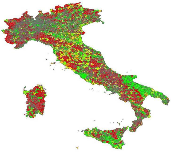
17B Orography and broadband in Italy
Figure 1: Percentage of the population covered by broadband in Italy.
Source: Between (2006), p. 17. Darker areas are those with the worst coverage.
Green areas have the best coverage.
18Figure 2: Topographic map of Italy.
19References
Angrist, J. D. (2001). Estimation of limited dependent variable models with
dummy endogenous regressors: simple strategies for empirical practice. Jour-
nal of business & economic statistics, 19(1):2–28.
Angrist, J. D. and Pischke, J.-S. (2009). Mostly harmless econometrics: an
empiricist’s companion. Princeton university press.
Antoci, A., Sabatini, F., and Sodini, M. (2015). Online and offline so-
cial participation and social poverty traps. Can social networks save hu-
man relations? Journal of Mathematical Sociology, 39(4):229 – 256. doi:
10.1080/0022250X.2015.1022278.
Arampatzi, E., Burger, M. J., and Novik, N. (2016). Social network sites,
individual social capital and happiness. Journal of Happiness Studies, pages
1–24.
Bartolini, S. and Sarracino, F. (2015). The dark side of Chinese growth: declin-
ing social capital and well-being in times of economic boom. World Develop-
ment, 74:333–351.
Bentham, J. (1781). An introduction to the principles of morals and legislation.
Reprinted Oxford: Clarendon Press, 1907.
Between (2006). Il punto sulla banda larga in Italia. Technical report, Osserva-
torio Banda Larga, Rome.
Bossert, W. and D’Ambrosio, C. (2006). Reference groups and individual de-
privation. Economics Letters, 90(3):421–426.
Brickman, P. and Bulman, R. J. (1977). Pleasure and pain in social comparison.
In J. Suls, Miller, R., editor, Social Comparison Processes: Theoretical and
Empirical Perspectives, pages 149–186. Washington, DC: Emisphere.
Brockmann, H., Delhey, J., Welzel, C., and Yuan, H. (2009). The China puzzle:
falling happiness in a rising economy. Journal of Happiness Studies, 10:387–
405.
Bruni, L. and Stanca, L. (2006). Income aspirations, television and happiness:
evidence from the World Values Survey. Kyklos, 59(2):209–225.
Campante, F. R., Durante, R., and Sobbrio, F. (2013). Politics 2.0: The mul-
tifaceted effect of broadband internet on political participation. Technical
report, National Bureau of Economic Research, w19029.
Chou, H.-T. G. and Edge, N. (2012). They are happier and having better lives
than I am: the impact of using Facebook on perceptions of others’ lives.
Cyberpsychology, Behavior, and Social Networking, 15(2):117–121.
20Ciapanna, E. and Sabbatini, D. (2008). La banda larga in Italia. Technical
report, Bank of Italy Occasional Papers, 34.
Clark, A. E. and Oswald, A. J. (1996). Satisfaction and comparison income.
Journal of Public Economics, 61(3):359–381.
Clark, A. E. and Senik, C. (2010). Who compares to whom? The anatomy of
income comparisons in Europe. The Economic Journal, 120(544):573–594.
Cohn, A., Fehr, E., Herrmann, B., and Schneider, F. (2014). Social compar-
ison and effort provision: evidence from a field experiment. Journal of the
European Economic Association, 12(4):877–898.
D’Ambrosio, C. and Frick, J. (2007). Income satisfaction and relative depriva-
tion: an empirical link. Social Indicators Research, 81(3):497–519.
D’Ambrosio, C. and Frick, J. (2012). Individual well-being in a dynamic per-
spective. Economica, 79:284–302.
de Vries, D. A. and Kühne, R. (2015). Facebook and self-perception: individual
susceptibility to negative social comparison on Facebook. Personality and
Individual Differences, 86:217–221.
Duesenberry, J. (1949). Income, savings and the theory of consumer behaviour.
Harvard Univesrity Press, Cambridge, MA.
Ellison, N. B., Steinfield, C., and Lampe, C. (2007). The benefits of Facebook
“friends”: social capital and college students’ use of online social network
sites. Journal of Computer-Mediated Communication, 12(4):1143–1168.
Ferrer-i Carbonell, A. (2005). Income and well-being: an empirical analysis of
the comparison income effect. Journal of Public Economics, 89(5-6):997 –
1019.
Festinger, L. (1954). A theory of social comparison processes. Human Relations,
7:117–140.
Frijters, P. and Leigh, A. (2008). Materialism on the march: from conspicuous
leisure to conspicuous consumption? Journal of Socio-Economics, 37:1937–
45.
Gamba, A., Manzoni, E., and Stanca, L. (2014). Social comparison and risk
taking behavior. Jena Economic Research Paper, 1.2014.
Guillen-Royo, M. (2017). Television, sustainability and happiness in Peru. TIK
Working papers on Innovation Studies 20171006, Centre for Technology, In-
novation and Culture, University of Oslo.
Guillen-Royo, M. and Kasser, T. (2015). Personal goals, socio-economic context
and happiness: Studying a diverse sample in Peru. Journal of Happiness
Studies, 16(2):405–425.
21Huang, L. and Shi, H. L. (2015). Keeping up with the Joneses: from conspicuous
consumption to conspicuous leisure? Oxford Economic Papers, 67(4):949–962.
Hyll, W. and Schneider, L. (2013). The causal effect of watching TV on material
aspirations: evidence from the “valley of the innocent”. Journal of Economic
Behavior & Organization, 86:37–51.
Kahneman, D., Wakker, P. P., and Sarin, R. (1997). Back to Bentham?
Explorations of experienced utility. The Quarterly Journal of Economics,
112(2):375–406.
Lewbel, A. (2012). Using heteroscedasticity to identify and estimate mismea-
sured and endogenous regressor models. Journal of Business & Economic
Statistics, 30(1):67–80.
Lim, M. and Yang, Y. (2015). Effects of users’ envy and shame on social com-
parison that occur on social network services. Computers in Human Behavior,
51:300–311.
Linde, J. and Sonnemans, J. (2012). Social comparison and risky choices. Jour-
nal of Risk and Uncertainty, 44(1):45–72.
Lohmann, S. (2015). Information technologies and subjective well-being: Does
the internet raise material aspirations? Oxford Economic Papers, 67(3):740–
759.
Marx, K. (1847). Wage, labour and capital. Transcripted in the Marx/Engels
Internet Archive (marxists.org).
Pempek, T. A., Yermolayeva, Y. A., and Calvert, S. L. (2009). College students’
social networking experiences on Facebook. Journal of Applied Developmental
Psychology, 30(3):227–238.
Sabatini, F. and Sarracino, F. (2017). Online networks and subjective well-
being. Kyklos, 70(3):456–480.
Stouffer, S., Suchman, E., DeVinney, L., Star, S., and Williams Jr, R. (1949).
The American soldier: adjustment during army life.(Studies in social psy-
chology in World War II), Vol. 1. Princeton Univ. Press.
Stutzer, A. (2004). The role of income aspirations in individual happiness.
Journal of Economic Behaviour & Organization, 54(1):89 – 109.
Tandoc, E. C., Ferrucci, P., and Duffy, M. (2015). Facebook use, envy, and
depression among college students: is facebooking depressing? Computers in
Human Behavior, 43:139–146.
Veblen, T. (1899). Theory of the Leisure Class: an economic study in the
evolution of institutions. Macmillan, New York.
22Wheeler, L. and Miyake, K. (1992). Social comparison in everyday life. Journal
of Personality and Social Psychology, 62(5):760–773.
Wills, T. A. (1981). Downward comparison principles in social psychology.
Psychological Bulletin, 90:245–271.
23Tables
Table 1: Descriptive statistics of variables in the Multipurpose Household Sur-
vey.
Variable mean sd min max obs
financial dissatisfaction 2.529 0.751 1 4 38812
online networking 0.460 0.498 0 1 38812
optic fiber (%) 91.52 7.202 73.01 99.64 38812
broadband coverage 89.07 6.102 68.60 97.30 38812
women 0.453 0.498 0 1 38812
age 38.98 13.24 18 89 38812
age squared/100 16.94 11.15 3.240 79.21 38812
frequency of meetings with friends 5.378 1.248 1 7 38661
minutes spent watching TV 4.895 0.550 2.303 6.802 29466
marital status 1.660 0.672 1 4 38812
educational status 2.990 0.711 1 5 38812
occupational status 1.932 1.539 1 7 38812
number of children 1.278 0.980 0 7 38812
modem 0.0903 0.287 0 1 33220
DSL 0.590 0.492 0 1 33220
fiber 0.0161 0.126 0 1 33220
satellite 0.0823 0.275 0 1 33220
3G 0.0267 0.161 0 1 33220
USB 0.175 0.380 0 1 33220
mobile 0.0198 0.139 0 1 33220
fast internet connection 0.606 0.489 0 1 33220
real GDP per capita (thousands e2005) 23.65 5.591 14.58 30.77 38812
internet penetration among families 53.40 4.978 44.09 61.83 38812
region – – 10 200 38812
year – – 2010 2012 38812
24Table 2: Descriptive statistics of variables in the Eurobarometer.
variable mean sd min max obs
financial dissatisfaction 2.374 0.756 1 4 94859
use of online social networks 3.178 2.216 1 6 83749
woman 0.536 0.499 0 1 96169
age 47.93 17.60 15 98 96169
age squared/100 26.07 17.47 2.250 96.04 96169
married 0.648 0.478 0 1 96801
divorced 0.0736 0.261 0 1 96801
widow 0.0846 0.278 0 1 96801
household income scale 5.476 1.662 1 10 94156
media use index 1.905 0.897 1 4 96149
secondary education 0.146 0.354 0 1 94478
tertiary education 0.101 0.301 0 1 94478
in education 0.0286 0.167 0 1 94478
no full-time education 0.00382 0.0617 0 1 94478
employed 0.438 0.496 0 1 96801
not working 0.488 0.500 0 1 96801
household size 2.576 1.084 1 4 96801
small or middle sized town 0.320 0.467 0 1 96491
large town 0.334 0.471 0 1 96491
log of GDP per capita 10.29 0.368 9.339 11.42 95900
year – – 2011 2013 95900
country – – 1 43 96823
25Table 3: Ordered probit regressions of SNS use on financial dissatisfaction using MHS data. Control variables are included
step-wise.
(1) (2) (3)
∗∗ ∗
women −0.0441 (−2.92) −0.0343 (−2.26) −0.0317∗ (−2.09)
age 0.0288∗∗∗ (6.93) 0.0278∗∗∗ (6.67) 0.0300∗∗∗ (7.18)
age squared/100 −0.0369∗∗∗ (−7.83) −0.0358∗∗∗ (−7.60) −0.0368∗∗∗ (−7.81)
good health 0.277 (1.35) 0.240 (1.16) 0.237 (1.15)
neither good nor bad health −0.0567 (−0.29) −0.0821 (−0.41) −0.0862 (−0.43)
bad health −0.347∗ (−1.77) −0.369∗ (−1.86) −0.371∗ (−1.88)
very bad health −0.514∗∗ (−2.61) −0.541∗∗ (−2.72) −0.545∗∗ (−2.75)
married −0.210∗∗∗ (−9.91) −0.225∗∗∗ (−10.56) −0.215∗∗∗ (−10.10)
separated or divorced 0.0262 (0.82) 0.0176 (0.55) 0.0188 (0.58)
widow −0.0859 (−1.28) −0.0992 (−1.47) −0.0936 (−1.38)
vocational education −0.199 (−0.93) −0.234 (−1.10) −0.266 (−1.22)
lower secondary education −0.340 (−1.60) −0.391∗ (−1.84) −0.424∗ (−1.96)
secondary education −0.520∗ (−2.44) −0.584∗∗ (−2.74) −0.618∗∗ (−2.85)
tertiary education −0.648∗∗ (−2.95) −0.718∗∗ (−3.25) −0.750∗∗∗ (−3.35)
unemployed 0.765∗∗∗ (28.53) 0.700∗∗∗ (25.67) 0.700∗∗∗ (25.68)
housewife 0.137∗∗∗ (4.14) 0.113∗∗∗ (3.40) 0.114∗∗∗ (3.45)
student 0.0581∗ (1.85) 0.0204 (0.65) 0.0180 (0.57)
disabled 0.321∗ (2.43) 0.288∗ (2.18) 0.291∗ (2.21)
26
retired −0.00854 (−0.23) −0.00157 (−0.04) −0.00331 (−0.09)
other work condition 0.363∗∗∗ (4.95) 0.344∗∗∗ (4.70) 0.345∗∗∗ (4.73)
number of children 0.0671∗∗∗ (8.42) 0.0517∗∗∗ (6.43) 0.0532∗∗∗ (6.62)
frequency of meetings with friends −0.0319∗∗∗ (−4.99) −0.0424∗∗∗ (−6.60) −0.0453∗∗∗ (−7.03)
minutes spent watching TV 0.0875∗∗∗ (6.34) 0.0703∗∗∗ (5.07) 0.0679∗∗∗ (4.90)
year 2010 −0.0341 (−1.29) −0.0194 (−0.69) −0.0206 (−0.73)
year 2011 −0.0301 (−1.14) −0.0240 (−0.90) −0.0279 (−1.05)
fast internet connection 0.0154 (0.62) 0.0347 (1.38) 0.0239 (0.95)
mobile −0.0500 (−0.84) −0.0313 (−0.52) −0.0486 (−0.81)
USB 0.0604∗ (2.09) 0.0639∗ (2.20) 0.0568∗ (1.95)
3G −0.0789 (−1.58) −0.0655 (−1.31) −0.0788 (−1.57)
satellite −0.0553 (−1.61) −0.0321 (−0.93) −0.0437 (−1.26)
real GDP per capita (thousands e2005) −0.0242∗∗∗ (−11.06) −0.0237∗∗∗ (−10.81)
internet penetration among families 0.00561∗ (2.22) 0.00517∗ (2.05)
online networking 0.107∗∗∗ (6.70)
cut1 −1.719∗∗∗ (−5.51) −2.261∗∗∗ (−6.80) −2.219∗∗∗ (−6.64)
cut2 0.295 (0.95) −0.234 (−0.71) −0.190 (−0.57)
cut3 1.418∗∗∗ (4.56) 0.894∗∗ (2.70) 0.939∗∗ (2.82)
Observations 25379 25379 25379
Pseudo R2 0.044 0.048 0.049
t statistics in parentheses
∗ p < 0.1, ∗∗ p < 0.01, ∗∗∗ p < 0.001You can also read