Lower-thermosphere-ionosphere (LTI) quantities: current status of measuring techniques and models - ANGEO
←
→
Page content transcription
If your browser does not render page correctly, please read the page content below
Ann. Geophys., 39, 189–237, 2021
https://doi.org/10.5194/angeo-39-189-2021
© Author(s) 2021. This work is distributed under
the Creative Commons Attribution 4.0 License.

Lower-thermosphere–ionosphere (LTI) quantities: current status of
measuring techniques and models
Minna Palmroth1,2 , Maxime Grandin1 , Theodoros Sarris3 , Eelco Doornbos4 , Stelios Tourgaidis3,5 , Anita Aikio6 ,
Stephan Buchert7 , Mark A. Clilverd8 , Iannis Dandouras9 , Roderick Heelis10 , Alex Hoffmann11 , Nickolay Ivchenko12 ,
Guram Kervalishvili13 , David J. Knudsen14 , Anna Kotova9 , Han-Li Liu15 , David M. Malaspina16,17 ,
Günther March18 , Aurélie Marchaudon9 , Octav Marghitu19 , Tomoko Matsuo20 , Wojciech J. Miloch21 ,
Therese Moretto-Jørgensen22 , Dimitris Mpaloukidis3 , Nils Olsen23 , Konstantinos Papadakis1 , Robert Pfaff24 ,
Panagiotis Pirnaris3 , Christian Siemes18 , Claudia Stolle13,25 , Jonas Suni1 , Jose van den IJssel18 , Pekka T. Verronen2,26 ,
Pieter Visser18 , and Masatoshi Yamauchi27
1 Department    of Physics, University of Helsinki, Helsinki, Finland
2 Space  and Earth Observation Centre, Finnish Meteorological Institute, Helsinki, Finland
3 Department of Electrical and Computer Engineering, Democritus University of Thrace, Xanthi, Greece
4 Royal Netherlands Meteorological Institute KNMI, Utrecht, the Netherlands
5 Space Programmes Unit, Athena Research & Innovation Centre, Athens, Greece
6 Space Physics and Astronomy Research Unit, University of Oulu, Oulu, Finland
7 Swedish Institute of Space Physics (IRF), Uppsala, Sweden
8 British Antarctic Survey (UKRI-NERC), Cambridge, UK
9 Institut de Recherche en Astrophysique et Planétologie, Université de Toulouse, CNRS, CNES, Toulouse, France
10 Center for Space Sciences, University of Texas at Dallas, Dallas, USA
11 European Space Research and Technology Centre, European Space Agency, Noordwijk, the Netherlands
12 Division of Space and Plasma Physics, Royal Institute of Technology KTH, Stockholm, Sweden
13 GFZ Potsdam, German Research Centre for Geosciences, Potsdam, Germany
14 Department of Physics and Astronomy, University of Calgary, Calgary, Canada
15 National Center for Atmospheric Research, Boulder, USA
16 Astrophysical and Planetary Sciences Department, University of Colorado, Boulder, USA
17 Laboratory for Atmospheric and Space Physics, University of Colorado, Boulder, USA
18 Faculty of Aerospace Engineering, Delft University of Technology, Delft, the Netherlands
19 Institute for Space Sciences, Bucharest, Romania
20 Ann and H.J. Smead Department of Aerospace Engineering Sciences, University of Colorado at Boulder, Boulder, USA
21 Department of Physics, University of Oslo, Oslo, Norway
22 University of Bergen, Institute of Physics and Technology, Bergen, Norway
23 DTU Space, Technical University of Denmark, Copenhagen, Denmark
24 Heliophysics Science Division, NASA/Goddard Space Flight Center, Greenbelt, USA
25 Faculty of Science, University of Potsdam, Potsdam, Germany
26 Sodankylä Geophysical Observatory, University of Oulu, Sodankylä, Finland
27 Swedish Institute of Space Physics (IRF), Kiruna, Sweden

Correspondence: Minna Palmroth (minna.palmroth@helsinki.fi)

Received: 25 June 2020 – Discussion started: 1 July 2020
Revised: 6 January 2021 – Accepted: 21 January 2021 – Published: 25 February 2021

Published by Copernicus Publications on behalf of the European Geosciences Union.
190                                                                 M. Palmroth et al.: LTI: measurements and modelling

Abstract. The lower-thermosphere–ionosphere (LTI) system             A few comprehensive reviews of the LTI have been pub-
consists of the upper atmosphere and the lower part of the        lished in the recent years. Vincent (2015) concentrates on the
ionosphere and as such comprises a complex system cou-            atmospheric dynamics within the region. Laštovička (2013)
pled to both the atmosphere below and space above. The at-        and Laštovička et al. (2014) review the trends in the obser-
mospheric part of the LTI is dominated by laws of contin-         vational state of the art within the upper atmosphere and
uum fluid dynamics and chemistry, while the ionosphere is         ionosphere. Sarris (2019) reviews the characterisation sta-
a plasma system controlled by electromagnetic forces driven       tus and presents the key open questions especially in terms
by the magnetosphere, the solar wind, as well as the wind         of measurement gaps within the LTI, while also highlight-
dynamo. The LTI is hence a domain controlled by many dif-         ing the discrepancies between observations and models. A
ferent physical processes. However, systematic in situ mea-       recently accepted review article by Heelis and Maute (2020)
surements within this region are severely lacking, although       describes the challenges within the understanding of the LTI
the LTI is located only 80 to 200 km above the surface of         in terms of coupling to the lower atmosphere, the LTI as a
our planet. This paper reviews the current state of the art       source of currents, its coupling to regions above, and the re-
in measuring the LTI, either in situ or by several different      sponse of the LTI to different drivers. Apart from these re-
remote-sensing methods. We begin by outlining the open            cent reviews, one of the most thorough introductions to the
questions within the LTI requiring high-quality in situ mea-      LTI dates back to a 1995 book within the American Geo-
surements, before reviewing directly observable parameters        physical Union Geophysical Monograph Series, reviewing,
and their most important derivatives. The motivation for this     among other aspects, the dynamics of the lower thermo-
review has arisen from the recent retention of the Daedalus       sphere (Fuller-Rowell, 2013). These reviews and scientific
mission as one among three competing mission candidates           studies published in the literature explain that the LTI is es-
within the European Space Agency (ESA) Earth Explorer 10          sentially a transition region with steep gradients in altitude:
Programme. However, this paper intends to cover the LTI pa-       the dominance of the neutral atmosphere decreases within the
rameters such that it can be used as a background scientific      LTI as evidenced by the decrease in the neutral density and
reference for any mission targeting in situ observations of the   the drastic increase in the temperature due to absorption of
LTI.                                                              solar extreme ultraviolet (EUV) radiation that occurs within
                                                                  the thermosphere. On the other hand, this is also the region
                                                                  where near-Earth space, controlled by electromagnetic ef-
                                                                  fects, starts to influence the overall dynamics as part of the
                                                                  neutrals are dissociated and the medium has the characteris-
1   Introduction                                                  tics of a plasma system. First and foremost, this suggests that
                                                                  the LTI is a region where the underlying physical processes
The region where the atmosphere meets space, consisting           change in nature, warranting understanding both from the at-
of the mesosphere and the lower thermosphere–ionosphere           mospheric perspective as well as in terms of space plasma
(LTI), is markedly difficult to measure directly and is there-    physics.
fore sometimes also termed the ignorosphere. The LTI re-             In the Earth’s denser lower atmospheric regions, up to the
gion, spanning from about 80 to 200 km in altitude, ex-           mesopause around 90 km altitude, the motion of the atmo-
hibits a relatively high atmospheric density, making system-      sphere is driven by the solar irradiance and the waves it pro-
atic satellite in situ measurements impossible from circu-        duces. The dynamics is typically described as a flow gov-
lar orbits. This is the region where de-orbiting spacecraft       erned by the laws of continuum fluid dynamics, for a gaseous
and orbital debris start to burn up while re-entering the at-     fluid that is electrically neutral. In the continuum assump-
mosphere. Hence sporadic rocket campaigns are currently           tion, averaging is performed over sampling volumes, such
the main source of in situ observations (e.g, Burrage et al.,     that the fluid particles are normally distributed and can thus
1993; Brattli et al., 2009). Remote optical observations re-      be described in terms of local bulk macroscopic properties,
quire measurable emissions reaching the remote detector;          notably pressure, temperature, density and flow velocity. The
however, there is a significant gap in ultraviolet, infrared,     continuum assumption requires the sampling volume to be
and optical emissions (for Fabry–Perot interferometers) at        in thermodynamic equilibrium, which implies a high fre-
approximately 100–140 km altitude, allowing only a part of        quency of collisions between atmospheric particles. Atmo-
the LTI to be measured remotely. Ground-based radar mea-          spheric flow is then predicted by solving the fundamental
surements are also inherently remote but are indispensable        conservation equations including the conservation of mass,
especially in characterising the ionised part of the LTI, the     momentum, and energy and a thermodynamic equation of
ionosphere. Due to the lack of systematic measurements, this      state. The energy from solar irradiance is mostly deposited
region still yields discoveries and surprises; for instance, as   as sensible and latent heat fluxes and via direct absorption of
recently reported by Palmroth et al. (2020), even citizen sci-    shortwave (solar) radiative energy, for instance by ozone in
entist pictures of the aurora may be relevant in obtaining new    the ozone layer and of re-radiated energy, typically by green-
information on the LTI.                                           house gases and clouds.

Ann. Geophys., 39, 189–237, 2021                                                  https://doi.org/10.5194/angeo-39-189-2021
M. Palmroth et al.: LTI: measurements and modelling                                                                           191

   Above the mesopause, neutral densities become so low           culation, chemistry, or the climate system (e.g. Gettelman
that collisions gradually become less important, while the        et al., 2019) normally do not take into account electromag-
density of the electrically charged ionospheric plasma in-        netic forces. On the other hand, the magnetosphere models
creases. In contrast to the atmospheric material, near-Earth      using a first-principle plasma approach, either using the mag-
space plasmas cannot be represented by a similar contin-          netohydrodynamics description (MHD; e.g. Janhunen et al.,
uum assumption due to the scarcity of collisions. The laws        2012; Glocer et al., 2013) or the (hybrid-)kinetic description
controlling plasma motion need to be incremented by elec-         (e.g. Omidi et al., 2011; Palmroth et al., 2018), have to be
tromagnetic forces, and thus the forcing from the magneto-        coupled to the ionosphere and neutral atmosphere. The iono-
sphere needs to be taken into account. At high latitudes, the     spheric first-principle (e.g. Marchaudon and Blelly, 2015;
ionosphere is coupled via the magnetic field to the magneto-      Verronen et al., 2005) or (semi-)empirical models (e.g. Bil-
sphere and even further into the solar wind. Further, plasma      itza and Reinisch, 2008) require coupling both to the mag-
particles are typically not normally distributed, implying that   netosphere and to the atmosphere. In the recent years, the
plasmas cannot be described by e.g. a single temperature. In      different modelling communities have started to integrate the
the transition region between the atmosphere described by         dedicated models towards new regimes; e.g. the Whole At-
the continuum dynamics and geospace described by plasma           mosphere Community Climate Model (WACCM) has been
kinetic theory, at altitudes roughly between 80 and 200 km,       extended to cover the thermosphere and ionosphere to about
the atmosphere starts to be significantly affected by the pres-   500 km altitude (WACCM-X Liu et al., 2018a). Likewise,
ence of the ionosphere. The neutral particles and plasmas in-     the Whole Atmosphere Model (WAM; e.g. Akmaev et al.,
teract through collisions and charge exchange, which max-         2008) and the Ground to topside model of the Atmosphere
imise at altitudes between 100 and 200 km but remain im-          and Ionosphere for Aeronomy (GAIA; e.g. Jin et al., 2012)
portant up to around 500 km altitude, the nominal base of         are coupled models of the neutral atmosphere and ionosphere
the exosphere, beyond which collisions are practically non-       suitable for studying the LTI dynamics. The MHD-based
existent.                                                         magnetospheric models have been coupled to the ionosphere
   Even though the LTI is characterised as a transition re-       and neutral atmosphere (Tóth et al., 2005). However, even
gion between the atmosphere and space, it is also markedly        though the models may currently be the main tool used to
a region with characteristics of its own. This is particularly    provide information on the coupled system, they can only be
true in terms of the energy sink that the region represents.      trusted after careful validation and verification. Hence, ulti-
From the atmospheric perspective, the energy of upward-           mately the only way to understand the LTI holistically is by
propagating atmospheric waves, such as planetary waves,           acquiring systematic measurements of the system.
tides, and gravity waves (for a review, see Vincent, 2015), is       There is a growing recognition that the Earth needs to be
deposited into the LTI. These waves can drive plasma insta-       studied and understood as a coupled system of its various
bilities, which in turn lead to small-scale variations that can   components. The European Space Agency’s (ESA) Living
cause disruption of radio signals (e.g. Xiong et al., 2016). On   Planet Programme embraces this need, calling for studies of
the other hand, at polar latitudes, the LTI is a major sink of    the many linkages within the system. From this viewpoint,
energy transferred from the solar wind by processes within        it follows that our understanding is only ever as good as the
the magnetosphere and ionosphere, which are not well un-          weakest link. One such weak link currently is the connection
derstood. In particular, during times of very large solar and     between the Earth and space. For example, there are con-
geomagnetic activity, for example as a response to interplan-     siderable changes caused by currents and energetic particles
etary coronal mass ejections (ICMEs, e.g. Richardson and          from outer space impinging on the atmosphere, and some
Cane, 2010) and stream interaction regions (SIRs) followed        of these changes are not well sampled and quantified at all,
by high-speed streams (HSSs, e.g. Grandin et al., 2019a),         leading to significant (and maybe even critical) uncertainties.
this energy input increases substantially and can represent a     ESA’s Earth Explorer 10 candidate mission Daedalus (Sarris
larger energy source than that provided by solar irradiance.      et al., 2020) has been designed to explore the LTI systemati-
Thus, the energetics, dynamics, and chemistry of the LTI          cally for the first time in situ to address the challenges within
result from a complex interplay of processes with coupling        the LTI described above.
both to the magnetosphere above and to the atmosphere be-            This paper introduces the science behind the Daedalus
low.                                                              candidate mission. First, we list the three main outstanding
   The neutral–plasma interactions and dynamics within the        topics under research, related to the LTI energy balance, LTI
LTI are poorly understood, mainly due to a lack of sys-           variability and dynamics, and LTI chemistry. The logic of
tematic observations of the key parameters in the region.         the paper is to present the outstanding science questions first
In the case of scarce observations, the solution is usually       with a short summarising background. These science top-
to build a model which can be used to obtain information          ics lead to the need of observing the key LTI parameters,
on the region. However, in the case of the LTI, this ap-          which are divided into those that can be observed directly
proach has been markedly difficult due to the complexity          and those that need to be derived from several other parame-
of the system: the atmospheric models solving general cir-        ters. The bulk of the review concentrates into these direct and

https://doi.org/10.5194/angeo-39-189-2021                                                   Ann. Geophys., 39, 189–237, 2021
192 M. Palmroth et al.: LTI: measurements and modelling
derived observables, while the science questions are on pur- 2.1 LTI energetics
pose concise, giving only a few central literature references.
An important choice made in this paper is related to the most In the following, LTI energetics refers to the energy input,
important energy deposition mechanism driven by the solar deposition, dissipation, and, in general, the energy balance
wind and magnetospheric forcing, called Joule heating. This within the LTI. Energetics is driven on the one hand by the
is such a vast topic that it requires a review of its own. How- solar radiative flux and on the other hand by energy depo-
ever, here the emphasis is on the parameters required to as- sition into the LTI from above (near-Earth space) and be-
sess Joule heating accurately. low (lower atmospheric regions). The solar radiative flux is
In the two most recent review papers of the LTI, Sarris mostly controlled by the inclination of the planet’s rotation
(2019) emphasises the main gaps in the current understand- axis with respect to the Sun-Earth line, as well as by the
ing of this key atmospheric region and discusses the related distance from the Sun. The energy input from below mainly
roadmaps and statements made by several agencies and other consists of atmospheric waves propagating upwards. The en-
international bodies, whereas Heelis and Maute (2020) pro- ergy input from above is extracted from the solar wind and
vide a detailed review of the physical processes and cou- processed by the magnetosphere, and it affects, e.g. the mo-
plings within the LTI. The purpose of this paper, in turn, is tion of the ionospheric charged particles and electromag-
to systematically list and discuss the parameters that can be netic fields within the LTI (e.g. Palmroth et al., 2004). There
observed or derived from in situ measurements, underlining are two primary energy sinks which deposit magnetospheric
the state of the art in observations and numerical models. The energy into the ionosphere, Joule heating (JH) and particle
intention is to give a background for the measurement setup (electron and proton) precipitation, of which the current un-
of any given future mission within the LTI, from the view- derstanding suggests that JH represents the larger sink (e.g.
point of the major outstanding questions. The paper is organ- Knipp et al., 1998; Lu et al., 1998). However, currently the
ised as follows: Sect. 2 presents the outstanding science ques- energy deposited per unit volume at LTI altitudes via JH and
tions related to the LTI. Sections 3 and 4 review the current particle precipitation is not known. Furthermore, the influ-
understanding of the LTI observed and derived parameters, ence of this energy deposition on the local transport, thermal
respectively, which are key to improve the understanding of structure, and composition within LTI altitudes is also poorly
the region and required to close the outstanding questions. known.
Section 5 ends the paper with concluding remarks.
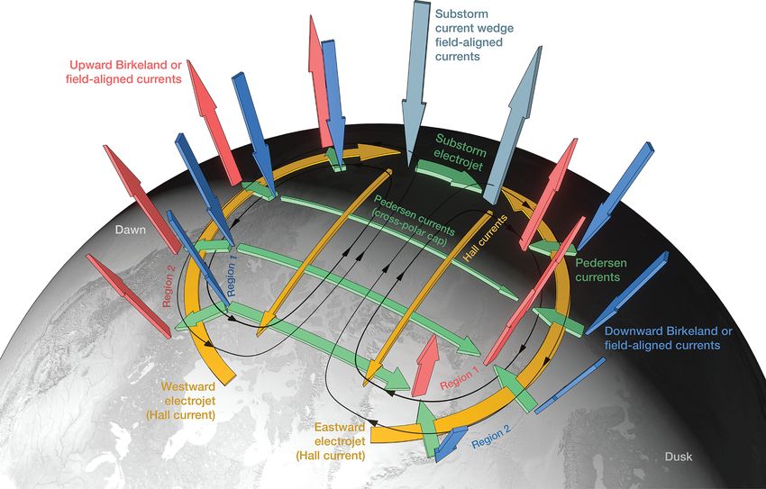
2.1.1 Joule heating
2 Open questions in LTI energetics, dynamics, and Joule heating is in general terms caused by electric currents
chemistry flowing through a resistive medium, which causes heating
within the medium. In the geospace, the current system con-
To assess the role of the LTI as a crucial component within
sists of field-aligned currents (FACs; see Sect. 4.2), which
the Earth’s atmospheric system, it is important to understand
find their closure through ionospheric horizontal currents in
the dominant processes involved in determining the energet-
the ionosphere (e.g. Sergeev et al., 1996), which is a resistive
ics, dynamics, and chemistry of the LTI. Such knowledge
medium as neutral and charged particles undergo collisions.
is also critical to develop capabilities to specify and fore-
Ultimately, the power density dissipated by JH is according
cast space weather phenomena that occur, originate and are
to Poynting’s theorem j · E, where j is the electric current
modified in this region. This section summarises these broad
density and E the electric field in the frame of the neutral
topics to give the background for the required observed and
gas. The electric field in the reference frame of the neutral
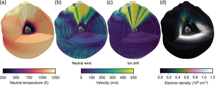
derived parameters outlined later. Figures 1 and 2 illustrate
gas, with a neutral gas velocity U 6 = 0, is E 0 = E + U × B
some of the crucial parameters in terms of energetics (tem-
with B the magnetic field (Kelley, 2009).
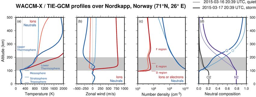
peratures in Figs. 1a and 2a), dynamics (neutral winds and
In this primary energy deposition mechanism, the addi-
ion drifts in Figs. 1b–c and 2b), and chemistry (electron den-
tional energy from the magnetosphere forces the plasma to
sity in Fig. 1d, ion/electron and neutral densities in Fig. 2c,
advect relative to the neutral gas, leading to ion–neutral fric-
and neutral composition in Fig. 2d), both over global scales
tional (or Joule) heating. During geomagnetic storms, current
in Fig. 1 and as altitude profiles near local magnetic midnight
knowledge indicates, albeit with large uncertainties, that this
during quiet and storm times in Fig. 2. In addition, Fig. 2 re-
energy sink is on a par with the heat created by absorption of
calls the usual nomenclature used in atmospheric and iono-
solar radiation, which otherwise is the major driver of atmo-
spheric studies, indicating the names of the atmospheric lay-
spheric dynamics (Knipp et al., 2005). The effects of moder-
ers alongside the temperature profiles (Fig. 2a) and the D,
ate to strong geomagnetic activity can be significant at mid
E, and F regions (or layers) in the ionosphere alongside the
and equatorial latitudes, as auroral JH can launch travelling
electron density profiles (Fig. 2c). The LTI is indicated with
ionospheric disturbances which can have measurable effects
a grey shading in the profiles, between the mesopause (near
down to equatorial latitudes (e.g. Zhou et al., 2016; de Jesus
100 km) and 200 km altitude.
et al., 2016). By enhancing the ion temperature, JH modifies
Ann. Geophys., 39, 189–237, 2021 https://doi.org/10.5194/angeo-39-189-2021
M. Palmroth et al.: LTI: measurements and modelling                                                                                     193

Figure 1. Overview of some key atmosphere/ionosphere parameters from the WACCM-X model: (a) neutral temperature, (b) neutral wind
magnitude and streamlines, (c) ion drift magnitude and streamlines, and (d) electron density. The model output is from a simulation of the
2015 St. Patrick’s Day storm, showing the simulated state of the atmosphere on 17 March 2015, 18:00 UTC, during a period of significant
high-latitude energy input. Slices through the model are shown at the top pressure level, at 0 and −90◦ longitude and at −1◦ latitude. The
meridional slice over the Greenwich meridian (top right of each sphere) shows a dusk profile, while the 90◦ west slice shows a noon profile.
Pressure-level geopotential heights from the model have been exaggerated by 50 times to show vertical detail; concentric circles indicate
heights of 100, 200, and 500 km.

Figure 2. Altitude profiles from the WACCM-X and TIE-GCM models of some key atmospheric parameters over Nordkapp (71◦ N, 26◦ E)
during quiet time (lighter curves) and during a geomagnetic storm (darker curves) near local magnetic midnight. (a) Neutral (blue) and
ion (red/orange) temperature. (b) Zonal neutral wind (blue) and ion drift (red/orange). (c) Neutral (blue) and electron (red/orange) density.
(d) Neutral composition (main species). The grey area corresponds to the LTI, between the mesopause and 200 km altitude.

the chemical reaction rates and thus the local chemical equi-            200 km altitude regions where it maximises, sampled over a
librium and ion and neutral composition. The way by which                broad range of atmospheric and geomagnetic conditions and
neutral winds, ion drifts and electric fields interplay to gen-          at a resolution that captures the key scales associated with
erate heating is largely unknown, primarily due to the lack              this heating process. JH can occur down to very fine scales
of co-located measurements of all key parameters involved.               during active aurora (Matsuo and Richmond, 2008), as in
Since the topic of JH is vast, it is left as a subject of a sub-         particular electric fields and plasma parameters are believed
sequent paper, while we cover some of the knowledge and                  to have such extremely low scales within the aurora; the rel-
open questions of JH in Sect. 4.7.                                       evant scales for JH can be derived via association with the
   To understand this energy deposition mechanism, it is im-             observed scales for auroral structures as obtained by optical
perative to explore the energy deposited into the LTI through            measurements and are on the order of ∼ 100 m (e.g. Dahlgren
JH, by simultaneously measuring the comprehensive set of                 et al., 2016). At the same time, observations indicate that
variables determining JH in the auroral latitudes and 100–               the power (amplitude squared) typically decreases with de-

https://doi.org/10.5194/angeo-39-189-2021                                                           Ann. Geophys., 39, 189–237, 2021
194                                                                   M. Palmroth et al.: LTI: measurements and modelling

creasing wavelengths; thus, to quantify the heating processes,     (30 < E < 1000 keV) deposit their energy through ionisa-
overall it is not necessary to measure electromagnetic fields      tion into the mesosphere, while the lower-energy ions (E <
and plasma parameters down to the smallest scales, which           1 MeV) and auroral electrons (E < 30 keV) impact the ther-
might also be practically difficult. It is therefore considered    mosphere. The local values of precipitation-induced heating
that a spatial resolution on the order of ∼ 1 km is sufficient     are however largely unknown, as its quantification proves
for resolving Joule heating on scales that can lead to signifi-    challenging due to the scarcity of suitable observations. De-
cant progress in process understanding and quantification as       tailed measurements of the energy spectrum and flux of par-
well as in modelling, globally and over long terms. On the         ticles passing through the thermosphere as a function of so-
other hand, enhanced spatial resolution down to ∼ 100 m,           lar/geomagnetic conditions are key to accurately quantify-
such as could possibly be obtained through sporadic burst-         ing the impact of precipitation on the climate system (see
mode capabilities of instruments, would enable the derivation      Sect. 2.3.1).
of scale-vs.-power relationship for JH, down to very small            To quantify the energy deposited into the LTI through par-
scales. One challenge lies in that, since the quantification of    ticle precipitation, it is necessary to measure the energy spec-
JH is significantly affected by the measurements of the Ped-       trum and flux of precipitating particles at the auroral latitudes
ersen conductivity (e.g. Palmroth et al., 2005), it is necessary   in regions where it maximises, sampled over a broad range
to also characterise how collision cross sections, frequencies,    of geomagnetic conditions, and at resolutions in energy and
and the resulting conductivities vary with altitude and condi-     pitch angle that capture the characteristic scales associated
tions in the LTI, by simultaneously measuring the compre-          with the heating, ionisation, and dissociation processes of
hensive set of variables determining these parameters over         interest. Further to the values of energies presented above,
the relevant altitudes and for a range of atmospheric and ge-      which determine the energy range of interest for ion and elec-
omagnetic conditions.                                              tron measurements in relation to precipitation-driven energy
                                                                   inputs, since the EPP energy spectra present strong spectral
2.1.2   Precipitation-driven energy input                          gradients and since spectral features convey information on
                                                                   the precipitating particles’ acceleration mechanisms (Newell
The second most important energy deposition mechanism              et al., 2009; Dombeck et al., 2018), high-energy spectra
is caused by particle precipitation, which is typically di-        should ideally have at least 128 channels (similar number
vided into two categories: lower-energy auroral (∼ 0.01–           to the DEMETER/IDP spectrometer; Sauvaud et al., 2006),
20 keV, mostly electron) precipitation, depositing energy          whilst the spectral energy resolution at low energies should
within ∼ 100–300 km altitude, and energetic (> 30 keV) par-        ideally be at least 20 %. Particle precipitation should be mea-
ticle precipitation (EPP), including relativistic (> 1 MeV) en-    sured with a spatial resolution of the order of 10 km or better,
ergies, consisting of energetic electrons and ions deposit-        based on the corresponding and related typical scales of high-
ing energy below ∼ 90 km altitude (Berger et al., 1970).           latitude structures such as auroral arcs (Miles et al., 2018). To
Auroral ion precipitation occurs, with the specificity of its      assess the local response and relative importance of JH and
own that precipitating protons can undergo multiple charge-        EPP in the LTI, it is necessary to simultaneously measure the
exchange interactions with atmospheric constituents on their       comprehensive set of corresponding changes in composition,
way down, leading to a spreading of the affected area (see the     flows, and temperatures with adequate temporal resolution to
special section by Galand, 2001). The sources of auroral pre-      capture the involved processes.
cipitation and EPP are particles both directly coming from
the Sun or accelerated by various processes in the magne-          2.1.3   Energetics driven by the neutral atmosphere
tosphere. Broadly speaking, auroral precipitation comprises
larger number fluxes (Newell et al., 2009), while EPP con-         There are several types of waves within the lower atmo-
sists of higher energies. Hence both affect the energy depo-       sphere which travel vertically towards the LTI and are ex-
sition within the LTI, the former through larger areas and the     pected to dissipate there. These waves couple with the neu-
latter through higher energies.                                    tral wind, temperature field, and density in the LTI. They are
   The energy input from particle precipitation is given by        also believed to seed plasma instabilities, especially in the
the energy of the incoming particles deposited via either dy-      low-latitude region, and the upward-propagating waves can
namical or chemical processes at the altitude of dissipation,      produce large shears that may affect the overall circulation
for example through electron temperature enhancement, ion-         within the LTI. In particular, gravity waves (see Sect. 4.9)
isation of neutrals, excitation of neutrals or ions, and dis-      contribute significantly to the LTI energetics. From a high-
sociation of molecular species producing chemical compo-           resolution WACCM simulation (with horizontal resolution
nents (see also Sect. 2.3). The altitude of maximum energy         of ∼ 25 km, Liu et al., 2014), it has been calculated that the
deposition by precipitation is determined by particle ener-        total upward energy flux by resolved waves at 100 km alti-
gies (e.g. Turunen et al., 2009, Fig. 3): relativistic ions (E >   tude is 100–150 GW (Liu, 2016), which is comparable to the
30 MeV) and electrons (E > 1 MeV) penetrate down to the            daily average JH power input (Knipp et al., 2004). This is
stratosphere, energetic ions (1 < E < 30 MeV) and electrons        likely an underestimation of the actual energy flux by gravity

Ann. Geophys., 39, 189–237, 2021                                                   https://doi.org/10.5194/angeo-39-189-2021
M. Palmroth et al.: LTI: measurements and modelling                                                                            195

waves, since waves with horizontal scales less than 200 km         ing et al., 2009), fast tail plasma flows (e.g. Angelopoulos
are poorly resolved due to numerical dissipation (or not re-       et al., 1994), dipolarisation of the tail magnetic field (e.g.
solved at all) in the model. Measurements of the related LTI       Runov et al., 2011), plasmoids launched tailwards (e.g. Ieda
neutral atmosphere parameters (primarily neutral winds, un ,       et al., 2001), and rapidly northward-propagating bright au-
neutral temperature, Tn and neutral mass density, ρ) sam-          roral emissions (e.g. Frey et al., 2004). It is not within the
pled at 10 km resolution would allow detection of small-scale      scope of this paper to review all the substorm-related sub-
neutral parameter variations as well as gravity waves and          tleties; rather our purpose here is to emphasise the role of
tides (e.g. Preusse et al., 2008; Gumbel et al., 2020). The        substorms as one of the chief magnetospheric drivers of LTI
energy deposition rate is also estimated based on parame-          energetics and dynamics. This driving is mostly manifested
terised gravity waves: the total wave energy deposition rate       as increased precipitating particle fluxes as well as intensified
at 100 km altitude is 35 GW, and 75 % of that comes from pa-       FACs.
rameterised and resolved gravity waves (Becker, 2017). The            Another broad category of magnetospheric drivers of the
role of the neutral atmosphere forcing in LTI energetics can       LTI consists of the various waves which modify the pro-
only be estimated, because there are no comprehensive and          ton and electron pitch angles such that the particles precipi-
systematic observations of the coupling between neutrals and       tate into the LTI. These waves have a multitude of drivers,
ions in the LTI.                                                   and their characteristics and role in driving the LTI vary
                                                                   greatly. For example, Alfén waves, driven by solar wind–
2.2     LTI variability and dynamics                               magnetosphere interactions, propagate into the LTI, trans-
                                                                   ferring energy and momentum as well as modifying LTI lo-
This section summarises typical phenomena of spatial and           cal plasma properties such as the density, temperature, and
temporal variability in the LTI region and mentions dynam-         conductance via the total electron content (e.g. Pilipenko
ical processes that lead to reorganisation of e.g. neutral or      et al., 2014; Belakhovsky et al., 2016). Various wave modes,
electron density, conductivity, or wind. We consider forcing       primarily ultra-low-frequency (ULF), very-low-frequency
from above, defined as variations driven by magnetospheric         (VLF), and electromagnetic ion cyclotron (EMIC) waves,
dynamics (Sect. 2.2.1). The current key scientific questions       drive energetic particle precipitation (Thorne, 2010, see
related to LTI variability and dynamics are to understand the      also Sect. 3.1), which drives chemistry changes in the LTI
ways in which the magnetosphere drives plasma motion in            (Sect. 2.3). The characteristics and propagation of these
the high-latitude LTI and how this motion affects the motion       waves are important unsolved problems; however, they are
of the neutrals. We also consider forcing from below through       well measured only on the ground (e.g. Sciffer and Waters,
atmospheric waves (Sect. 2.2.2). In this topic, the current key    2002; Engebretson et al., 2018; Graf et al., 2013; Manninen
research question is to understand how large shears, sharp         et al., 2020) or above the LTI around 400 km altitude (e.g.
gradients, and small-scale plasma instabilities develop in the     Li and Hudson, 2019). To build a complete picture of wave
LTI in response to driving from below. LTI variability and dy-     propagation through the LTI, direct in situ measurements of
namics take a special form at the low geomagnetic latitudes,       these waves are required simultaneously with the plasma and
summarised in Sect. 2.2.3. At low latitudes, the current key       neutral gas parameters, which determine the wave propaga-
scientific question is to quantify the relative contributions of   tion in this region. To analyse Alfvén waves and the Poynt-
magnetospheric, solar and atmospheric forcing influencing          ing flux, both electric and magnetic fields should be simul-
LTI fluid dynamics and electrodynamics.                            taneously sampled and at the same cadence. Furthermore,
                                                                   the spectra of measured electric fields should span the entire
2.2.1    LTI forcing from above                                    range of waves that are related to mechanisms important for
                                                                   energy exchange and heating in the lower ionosphere, includ-
Magnetospheric driving of the LTI can take the form of elec-       ing two-stream waves, Alfvén waves, ion cyclotron waves,
tromagnetic driving due to rapid variations in the geomag-         lightning-induced sferics and whistlers, lower hybrid waves,
netic field and wave–particle interactions within the mag-         solitary structures, power line radiation and Schumann res-
netosphere. Both processes involve the geomagnetic field           onances, as well as various high-frequency (HF) modes. To
(Sect. 3.6) and FACs (Sect. 4.2). The geomagnetic field vari-      study wave–particle interactions, the ambient ion cyclotron
ations are chiefly due to substorms which are often defined        frequencies and their harmonics should be covered with elec-
as periods of solar wind energy loading and subsequent mag-        tric field and density wave measurements. It is noted that,
netospheric unloading (e.g. McPherron, 1979). While there          while obtaining the power spectral density of the AC elec-
is still much debate about the sequence of events that lead to     tric field enables the broad characterisation of the variations
a substorm onset (e.g. Angelopoulos et al., 2008; Lui, 2009),      in the power of these waves, the continuous high sampling
from the phenomenological perspective it is agreed that sub-       of the DC-coupled and AC electric field time series is essen-
storms involve magnetotail reconnection (e.g. Angelopoulos         tial for revealing the detailed waveforms and their non-linear
et al., 2008), a FAC system connecting the tail plasma sheet       steepening due to heating, as well as their modulation associ-
to the ionosphere called substorm current wedge (e.g. Keil-        ated with precipitating auroral electrons and their behaviour

https://doi.org/10.5194/angeo-39-189-2021                                                    Ann. Geophys., 39, 189–237, 2021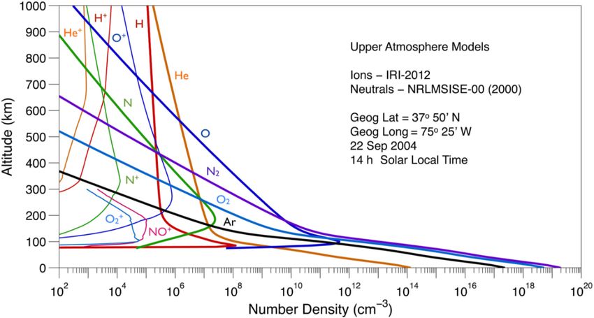
196                                                                   M. Palmroth et al.: LTI: measurements and modelling

at the edges of rapidly changing plasma density gradients,         corresponding local changes in composition, densities, and
structures, and depletions.                                        temperatures at the relevant latitudes and altitudes, sampled
   Downward LTI forcing is not limited to processes origi-         over a range of atmospheric and geomagnetic conditions and
nating from the magnetosphere. Solar flares are also known         at temporal scales that capture the key processes involved, in-
to enhance electron density and hence JH in the LTI (e.g. Pu-      cluding gravity waves, planetary waves, and tides originating
dovkin and Sergeev, 1977; Sergeev, 1977; Curto et al., 1994;       from the lower atmosphere. As in Sect. 2.1.3 above, sampling
Yamazaki and Maute, 2017). While the solar-flare-driven            at 10 km resolution would allow the detection of even small-
ionospheric current, or crochet current, near the subsolar         scale variations as well as gravity waves and tides (Preusse
region has been intensively studied (e.g. Annadurai et al.,        et al., 2008; Gumbel et al., 2020).
2018), its counterpart at high latitudes has been poorly un-
derstood for 40 years, although it significantly enhances pre-     2.2.3   Variability and dynamics in the low-latitude LTI
existing JH at the auroral electrojets (Pudovkin and Sergeev,
1977). The modification of the auroral electrojets by solar        At low latitudes, the dynamics of the LTI, comprising the
flares can be more than a mere enhancement. Recently, Ya-          ionosphere E region and lower F region, determines signif-
mauchi et al. (2020) found that the solar flares can change the    icant parts of the variability of the entire thermosphere and
direction of the electrojet, and the resulting geomagnetic de-     ionosphere through global electric field variations (Scherliess
viation sometimes exceeds 200 nT. The European Incoherent          and Fejer, 1999) and related large- to medium-scale plasma
Scatter (EISCAT) radar observation suggested that even the         transport, the most important phenomenon being known as
altitude of JH can be changed for these events. It is quite pos-   the equatorial ionisation anomaly (e.g. Walker et al., 1994;
sible that the altitude of the ionospheric current also changes,   Stolle et al., 2008b). The E-region dynamo which results
but no measurement method to prove this has been proposed.         from charged particles transported by thermospheric winds
   To understand the forcing from above, it is necessary to        through the nearly horizontal magnetic field (e.g. Heelis,
explore the momentum transfer between the plasma and the           2004) is understood to play a key role in driving the elec-
neutral fluid in the LTI, by simultaneously measuring the          tric fields and the equatorial electrojet, the latter being a rib-
comprehensive set of variables determining the forces glob-        bon of strong eastward dayside current flowing along the
ally, sampling a broad range of atmospheric and geomagnetic        magnetic equator. While the general principles are described,
conditions, and over timescales that capture the involved pro-     the significant day-to-day variability of their magnitudes is
cesses.                                                            still the subject of investigation (e.g. Yamazaki and Maute,
                                                                   2017). A special category of the LTI variability and dynam-
2.2.2   LTI forcing from below                                     ics within the low latitudes are post-sunset F-region equato-
                                                                   rial plasma irregularities, in which the LTI and lower F re-
Ionised gas under the influence of the geomagnetic field af-       gion are believed to play an important role. Suggested initial
fects greatly the overall dynamics of the LTI, which makes         perturbations for these plasma irregularities are the variabil-
it distinct, but not decoupled, from the atmosphere. In addi-      ity of the vertical plasma drift at sunset hours (e.g. Huang,
tion to Joule heating, the electromagnetic coupling asserts the    2018; Wu, 2015; Stolle et al., 2008a) and the role of upward-
Lorentz force acting on the ionised gas, providing geospace        propagating gravity waves (e.g. Krall et al., 2013; Hysell
with a lever on the atmosphere and also providing a lever          et al., 2014; Yokoyama et al., 2019; Huba and Liu, 2020). The
between hemispheres connected by the dipolar geomagnetic           resulting F-region plasma irregularities cause severe effects
field. Furthermore, the electromagnetic forcing affects and is     on trans-ionospheric radio wave signal propagation, leading
affected by atmospheric variations and disturbances, e.g. by       occasionally to “loss of lock” of space-borne global navi-
planetary (Rossby) waves, gravity waves, and solar or lunar        gation satellite system (GNSS) receivers (e.g. Xiong et al.,
tides, originating from below the LTI and propagating up-          2016; Xiong et al., 2020), and are thus an important source
wards. Many outstanding issues remain in our understanding         of space weather disturbances.
of the complex large-scale and global interactions between            To understand the LTI behaviour within low latitudes, it is
these processes and forces that act together to determine LTI      imperative to reveal the morphology of flow shears and sharp
dynamics. Especially the occurrence of strong flow shears,         gradients in the LTI and their role in driving plasma irregular-
steep gradients or rapid variations in the LTI parameters have     ities by simultaneously measuring the comprehensive set of
been observed but not been studied systematically due to a         variables that fully describe the LTI, including plasma den-
lack of consistent measurements of the relevant parameters.        sity at a resolution that captures the relevant processes, sam-
Consequently, the effects of such structures on the LTI dy-        pled over a wide range of latitudes and altitudes. Since the
namics are not well known. The physics of the different at-        Fresnel scale length that is found to be critical in creating ra-
mospheric waves is reviewed in Sect. 4.9.                          dio wave scintillations, such as on Global Positioning System
   To understand the driving from below, it is necessary to si-    (GPS) or other kinds of GNSS, is lower than 500 m (Kintner
multaneously measure all the variables defining not only the       et al., 2007), resolving density structures of less than 500 m,
neutral dynamics, but also the electrodynamics as well as the      e.g. up to 50 m, covers the pertinent range of scales well.

Ann. Geophys., 39, 189–237, 2021                                                    https://doi.org/10.5194/angeo-39-189-2021
M. Palmroth et al.: LTI: measurements and modelling 197
2.3 LTI chemistry resolution would allow the detection of the boundaries of pre-
cipitation regions such as auroral arcs (Miles et al., 2018).
The chemical composition of the LTI may change in re- The LTI region chemistry is recognised to be important for
sponse to particle precipitation (Sect. 2.3.1), temperature in- long-term climate simulations due to its role in solar-driven
crease associated with frictional/Joule heating (Sect. 2.3.2), NOx production and ozone impact (Matthes et al., 2017).
and through chemical heating (Sect. 2.3.3) resulting from However, there are substantial differences between simulated
exothermic reactions. The current key science questions in and observed distributions of polar NOx , owing partly to an
upper atmospheric chemistry are related to the chemical ef- incomplete representation of electron precipitation (Randall
fects of EPP within the mesosphere (and the stratosphere be- et al., 2015). Further, adequate climate simulations require
low) as a function of geomagnetic driving conditions. Fur- a NOx upper boundary condition as well as a representation
ther, the role of driving conditions from below, including the of the dynamical–chemical coupling between thermospheric
upward-propagating gravity waves, in influencing the LTI NOx and stratospheric ozone. For so-called high-top models,
chemistry is not known. Finally, it is not known whether with upper boundary in the thermosphere, the boundary con-
the current model boundary conditions (see below) provide ditions can be defined by empirical models based on satellite
a good representation of the LTI physics as a function of data (e.g. Marsh et al., 2004), which depend on geomagnetic
LTI conditions and solar activity. This section is dedicated indices, day of the year, and solar flux. However, current
to summarising the background to these topics. models are based on temporally limited data and do not cover
full solar cycles and/or differences between solar cycles, and
2.3.1 Precipitation-driven chemistry recent studies indicate a need for improvements (Hendrickx
et al., 2018; Kiviranta et al., 2018). To improve the model
Electron and ion precipitation ionise and dissociate neu- boundary conditions, it is necessary to make observations of
trals through collisions (Sinnhuber et al., 2012). This has a NOx in the polar lower mesosphere below 150 km to charac-
direct effect in the atmospheric chemical composition via terise the NO reservoir and variability. Preferably, the mea-
ion chemistry which leads to production of odd hydrogen surements should be carried out long enough to cover the so-
(HOx ) and nitrogen (NOx ) (e.g. Codrescu et al., 1997; Sep- lar cycle and different EPP events to improve understanding
pälä et al., 2015). Considering the LTI coupling to the lower of the drivers for the climate model boundary conditions.
atmosphere, odd nitrogen (NOx =NO + NO2 ) is particularly
important because it has a long (∼ months) chemical life- 2.3.2 Heating-driven chemistry
time in polar winter conditions, and it descends to meso-
spheric and stratospheric altitudes down to ∼ 35 km (Ran- Changes in the ion and neutral temperatures, for instance as-
dall, 2007; Funke et al., 2014; Päivärinta et al., 2016) and sociated with ion–neutral frictional heating, affect the chem-
catalytically destroys ozone (Damiani et al., 2016; Anders- ical reaction rates in the LTI and can consequently modify
son et al., 2018). Ozone is an effective absorber of solar ul- the LTI composition. Grandin et al. (2015) found that during
traviolet radiation, and its variability modulates the thermal high-speed-stream-driven geomagnetic storms the auroral-
balance of the middle atmosphere and polar vortex dynam- oval F-region peak electron density can decrease by up to
ics (Brasseur and Solomon, 2005). These perturbations can 40 % in the evening magnetic local time (MLT) sector, es-
propagate to surface levels and modulate regional patterns of pecially around the equinoxes. The suggested mechanism to
temperatures and pressures (Gray et al., 2010; Seppälä et al., account for this electron density decrease is that ion–neutral
2014). Investigation of atmospheric reanalysis datasets and frictional heating associated with substorm activity may in-
coupled-climate model runs has shown that NOx and HOx crease the ion and neutral temperatures on timescales much
have the potential to modify regional winter-time surface less than an hour, resulting in an enhancement of the elec-
temperatures by as much as ±5 K by re-distributing annular tron loss rate by increasing both the chemical reaction rates
mode patterns at mid to high latitudes in both the Northern (functions of the ion temperature) and the molecular densi-
Hemisphere and Southern Hemisphere (Seppälä et al., 2009; ties by upwelling of the neutral atmosphere associated with
Baumgaertner et al., 2011). To understand these questions, it the neutral temperature increase. A subsequent study by Mar-
is necessary to make simultaneous observations of the EPP chaudon et al. (2018) confirmed that this mechanism, espe-
flux, energy spectral gradients, ion composition, and NOx cially through the latter process, can account for the long-
and measure EPP fluxes with good resolution in the energy lasting F-region peak reduction. Heating-driven composition
and pitch angle. Further, the involved energy spectral gradi- changes in the LTI have also been revealed in association
ents need to be described, along with the energy ranges that with subauroral polarisation streams (SAPS; e.g. Wang et al.,
cover the deposition altitudes from the lower thermosphere 2012) and solar proton events (e.g. Roble et al., 1987). How-
to the mesosphere down to the stratopause. These measure- ever, not many studies discuss heating-driven chemistry in
ments need to be sampled at rates fast enough to resolve dif- the LTI, indicating a lack of systematic measurements. Com-
ferent precipitation mechanisms and boundaries on scales of position, density and temperature observations sampled at
10 km or smaller. As in Sect. 2.1.2 above, sampling at 10 km ∼ 10 km resolution would allow the study of heating-driven
https://doi.org/10.5194/angeo-39-189-2021 Ann. Geophys., 39, 189–237, 2021198 M. Palmroth et al.: LTI: measurements and modelling
chemistry at regional scales (comparable to that studied in Particles (electrons and ions) precipitate into the LTI when
Grandin et al., 2015; Marchaudon et al., 2018), as well as they are scattered into the bounce loss cone. Pitch-angle scat-
the detection of the boundaries of precipitation regions asso- tering can be due to the magnetic field curvature radius being
ciated with substorms, subauroral polarisation streams, and close to the particle gyroradius (Sergeev and Tsyganenko,
solar proton events. 1982) or to wave–particle interactions. For instance, lower-
band chorus waves, often present in the morningside and
2.3.3 LTI chemistry and chemical heating dayside magnetosphere, can lead to energetic (E > 30 keV)
electron precipitation (Thorne et al., 2010), whereas EMIC
Chemical heating is one of the main energy sources in the waves can be efficient in scattering kiloelectronvolt protons
LTI, together with Joule heating, EUV radiation and parti- and megaelectronvolt electrons into the bounce loss cone
cle precipitation heating, resulting from the storage in latent (Rodger et al., 2008; Yahnin et al., 2009). Other suggested
chemical form and subsequent release of energy (Beig, 2003; pitch-angle scattering waves include the plasmaspheric hiss,
Beig et al., 2008). Chemical heating influences the upper at- which may contribute to the precipitation of subrelativistic
mosphere in a variety of ways, including the formation of electrons (He et al., 2018). Phenomena such as pulsating au-
mesospheric inversion layers (Ramesh et al., 2013). Chem- rora have been found to be associated with precipitating elec-
ical energy is deposited in the LTI through the exothermic trons across a wide range of energies (e.g. Grandin et al.,
reactions typically involving oxygen (atomic and molecu- 2017b; Tsuchiya et al., 2018), which suggests interaction
lar) and ozone (e.g. Singh and Pallamraju, 2018). Neutral with whistler chorus waves (Miyoshi et al., 2015) or elec-
species, namely O3 , H2 O, CO2 , OH, and aerosols, are be- trostatic electron cyclotron harmonic waves (Fukizawa et al.,
lieved to play a role both in the chemistry of the LTI and in 2018). Evaluating the relative contribution of each scattering
the radiative balance of the mesosphere (Mlynczak, 2000). process to the global precipitation budget is challenging; ob-
On the other hand, CO2 molecules can induce radiative cool- taining particle measurements at multiple pitch angle values
ing in the LTI through their emission at 15 µm. Especially in the bounce loss cone with good energy resolution across
between 75 and 110 km altitude, this emission is the only the energy range could prove decisive in this endeavour.
significant cooling mechanism (e.g. Fomichev et al., 1986), Precipitating particles can have energies ranging from tens
while below, radiative cooling by ozone and H2 O is also im- of electronvolt to tens of megaelectronvolt. While low-energy
portant (e.g. Bi et al., 2011). Quantifying the contribution (E ≈ 0.1–30 keV) electrons and protons primarily precipi-
of chemical heating to the changes in the LTI composition tate at high latitudes, in the polar cusps and in the night-
is vital in order to understand the full radiative balance of side auroral oval (which is usually above ∼ 65◦ geomagnetic
the upper atmosphere. Furthermore, the spatial and tempo- latitude), relativistic electrons from the outer radiation belt
ral distributions of neutral species could be used as tracers (E ≈ 0.1–10 MeV) mostly precipitate at subauroral latitudes,
of wave and tidal phenomena (Solomon and Roble, 2015), i.e. equatorwards from the auroral oval. Solar energetic par-
which affect the overall dynamics of the LTI. Therefore, it ticles (E > 10 MeV protons), on the other hand, precipitate
is important to obtain measurements of the chemical com- directly from the solar wind into the polar region (geomag-
position and heating in the LTI. Measuring the neutral tem- netic latitudes above ∼ 60◦ ); however, the largest of those
perature and composition at ∼ 10 km resolution would allow events are rare and typically occur only a few times per so-
the detection of regions experiencing chemical heating. To- lar cycle (Neale et al., 2013). Energetic neutral atoms (1–
gether with EPP measurements at the same spatial resolution 1000 keV, principally within the 100 keV range; Orsini et al.,
(see Sect. 2.1.2) and numerical models of mesosphere and 1994; Roelof, 1997; Goldstein and McComas, 2013) are pro-
lower-thermosphere chemistry, this would enable the study duced via charge exchange when energetic ions interact with
of the role of each neutral species in chemical heating and in background neutral atoms such as Earth’s geocorona. They
the radiative balance of this atmospheric region. can play a role in mass and energy transfer to lower lati-
tudes beyond the auroral zone (Fok et al., 2003) and become
3 Observed LTI parameters: current understanding strongly coupled to precipitating energetic ions in the lower
thermosphere (Roelof, 1997).
3.1 Precipitating particle fluxes and energies To date the most comprehensive measurements of parti-
cle distributions in the near-Earth environment have been
Particle precipitation is very much connected to the overall made by flagship spacecraft missions such as DEMETER
electrodynamic coupling within the LTI. Precipitation leads (Sauvaud et al., 2006), Cluster (Escoubet et al., 2001), Mag-
to increased ionospheric conductivities (Aksnes et al., 2004) netospheric Multiscale (MMS; Burch et al., 2016), Arase
and creates FACs (see Sect. 4.2). FACs close in the E region (Miyoshi et al., 2018), and the Van Allen Probes (Mauk et al.,
of the ionosphere, leading to ion–neutral frictional heating 2013). However, at high altitudes, bounce loss cone angles
(Millward et al., 1999; Redmon et al., 2017, see Sect. 4.7). have values on the order of a few degrees only, which is
Since it plays such a leading role in the electrodynamic cou- too small to be resolved by most particle instruments carried
pling, we discuss precipitation first. by those spacecraft. On the other hand, at altitudes where
Ann. Geophys., 39, 189–237, 2021 https://doi.org/10.5194/angeo-39-189-2021M. Palmroth et al.: LTI: measurements and modelling 199
low-Earth orbit (LEO) satellites fly, the bounce loss cone 2014) was developed to predict auroral power as a function of
at auroral latitudes has its edges at an angle of about 60◦ solar wind parameters. This model separates auroral precipi-
from the magnetic field direction (Rodger et al., 2010a); it tation into four types (diffuse, monoenergetic, broadband and
is therefore possible to resolve it with particle detectors. A ion); Fig. 3b gives an example of output of the diffuse auroral
large number of LEO spacecraft missions have flown par- precipitation, obtained during the conditions when the dif-
ticle detectors measuring differential and integral precipita- ferential flux shown in Fig. 3a was observed. For higher en-
tion fluxes. The Solar, Anomalous, and Magnetospheric Par- ergies, while the AE-8 (electrons) and AP-8 (protons) maps
ticle Explorer (SAMPEX; Baker et al., 1993) mission (1992– provide trapped fluxes in the radiation belts (Vette, 1992), the
2012) produced megaelectronvolt electron precipitation data models developed by van de Kamp et al. (2016) and van de
that have been used in scientific studies (e.g. Blum et al., Kamp et al. (2018) predict 30–1000 keV electron precipita-
2015). The SSJ experiment aboard Defense Meteorological tion fluxes as a function of the Ap index based on analysing
Satellite Program (DMSP) satellites has provided precipitat- energetic electron precipitation observed by POES satellites
ing proton and electron observations in up to 20 channels during 1998–2012. Such climatologies prove particularly
covering the lower energies (30 eV–30 keV) since 1974 (e.g. useful for space weather predictions and can be used as in-
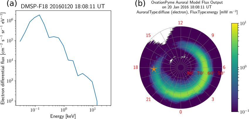
Hardy et al., 1984; Redmon et al., 2017); Figure 3a gives puts to ionospheric models, such as the IRAP Plasmasphere-
an example of differential number flux of precipitating elec- Ionosphere Model (IPIM; Marchaudon and Blelly, 2015) or
trons measured by DMSP-F18 on 20 January 2016 in the WACCM (Kinnison et al., 2007). Finally, a few attempts to
evening sector of the northern auroral oval. Higher-energy model particle precipitation in global, first-principle simula-
(> 30 keV) precipitation observations have on the other hand tions of the near-Earth environment have been made, in mag-
been routinely provided by NOAA Polar-orbiting Opera- netohydrodynamics models (e.g. Palmroth et al., 2006a), in
tional Environmental Satellite Space Environment Monitor some cases coupled with a test-particle code (e.g. Connor
(POES/SEM) instrument suite since 1979, although mea- et al., 2015), as well as in hybrid-particle-in-cell simulations
surements have suffered from contamination issues that were (e.g. Omidi and Sibeck, 2007) and more recently using a
corrected by Asikainen and Mursula (2013). Particle detec- hybrid-Vlasov model (Grandin et al., 2019b, 2020).
tors can nowadays even be included in nanosatellite mis-
sions; one example of upcoming CubeSat missions aimed 3.2 Temperatures
to measure particle precipitation is FORESAIL-1 (Palmroth
et al., 2019), which is expected to measure energetic and rel- The LTI temperature is a key background parameter, not only
ativistic electrons and protons. because it is a state parameter for the thermosphere itself,
Indirect observations of particle precipitation can be but it is also key in ultimately driving neutral winds and at-
achieved through various types of observations. Bal- mospheric expansion, as well as determining conditions for
loon experiments flying in the stratosphere can detect chemical reactions. While ion and electron temperatures, Ti
Bremsstrahlung emission produced by precipitating particles and Te , can exceed the neutral temperature Tn by thousands
interacting with neutrals in the atmosphere, as is done dur- of Kelvin (see Fig. 2a showing neutral and electron tempera-
ing BARREL campaigns (Woodger et al., 2015). Energetic ture profiles at selected latitudes obtained from a WACCM-X
electron precipitation is routinely monitored from the ground simulation), the largest thermal energy reservoir in the LTI is
using riometers, which measure the cosmic noise absorption in the neutral gas simply because of the low degree of ioni-
in the D region of the ionosphere associated with particle sation in the LTI (see Fig. 4). The largest heat production is
precipitation (e.g. Hargreaves, 1969; Rodger et al., 2013; by absorption of solar EUV and UV radiation which is ion-
Grandin et al., 2017a). Phase and amplitude perturbations ising and dissociating molecules. This process accounts for
to subionospheric man-made narrow-band transmitter sig- the well-known basic vertical structure of Tn and the thermo-
nals propagating over long distances are also routinely used spheric chemical composition.
to identify energetic electron precipitation (Clilverd et al., Reliable measurements of Tn have been difficult and less
2009). Incoherent scatter radar observations can be used to abundant compared to those of the neutral density itself
retrieve precipitating electron energy spectra (Virtanen et al., where especially the analysis of drag on satellite orbits has
2018) and to monitor the ionospheric impact of particle pre- boosted the available data in the recent decades. In diffusive
cipitation (Verronen et al., 2015). equilibrium (for each gas component) the profiles of den-
Empirical models have been developed by deriving statis- sity and Tn are not independent. Early models of the ther-
tical patterns of particle precipitation as a function of geo- mosphere were based on this assumption and an empirical
magnetic activity based on several years of spacecraft ob- formula, sometimes called the Bates profile:
servations. The Hardy model (Hardy et al., 1985, 1989) was
z − z0
established by compiling 2 years of DMSP measurements of Tn (z) = T∞ − T∞ − Tz0 exp − , (1)
H
precipitation and provides differential number fluxes of pre-
cipitating electrons and protons as a function of the Kp index. with T∞ the exospheric temperature, Tz0 the temperature at
More recently, the OVATION-Prime model (Newell et al., the base, z0 the height of the base, and H a scale height
https://doi.org/10.5194/angeo-39-189-2021 Ann. Geophys., 39, 189–237, 2021You can also read