100 years of progress in understanding the stratosphere and mesosphere
←
→
Page content transcription
If your browser does not render page correctly, please read the page content below
100 years of progress in understanding
the stratosphere and mesosphere
Article

Published Version

Baldwin, M. P., Birner, T., Brasseur, G., Burrows, J., Butchart,
N., Garcia, R., Geller, M., Gray, L., Hamilton, K., Harnik, N.,
Hegglin, M. I., Langematz, U., Robock, A., Sato, K. and
Scaife, A. (2018) 100 years of progress in understanding the
stratosphere and mesosphere. Meteorological Monographs,
59. 27.1-27.62. ISSN 1943-3646 doi:
https://doi.org/10.1175/amsmonographs-d-19-0003.1 Available
at http://centaur.reading.ac.uk/87003/

It is advisable to refer to the publisher’s version if you intend to cite from the
work. See Guidance on citing .

To link to this article DOI: http://dx.doi.org/10.1175/amsmonographs-d-19-0003.1

Publisher: American Meteorological Society

All outputs in CentAUR are protected by Intellectual Property Rights law,
including copyright law. Copyright and IPR is retained by the creators or other
copyright holders. Terms and conditions for use of this material are defined in
the End User Agreement .

www.reading.ac.uk/centaur

CentAUR

Central Archive at the University of Reading
Reading’s research outputs online
CHAPTER 27                                                 BALDWIN ET AL.                                                                     27.1

                                                                Chapter 27

            100 Years of Progress in Understanding the Stratosphere and Mesosphere

   MARK P. BALDWIN,a THOMAS BIRNER,b GUY BRASSEUR,c JOHN BURROWS,d NEAL BUTCHART,e
     ROLANDO GARCIA,f MARVIN GELLER,g LESLEY GRAY,h KEVIN HAMILTON,i NILI HARNIK,j
MICHAELA I. HEGGLIN,k ULRIKE LANGEMATZ,l ALAN ROBOCK,m KAORU SATO,n AND ADAM A. SCAIFEe
                a
                    Department of Mathematics and Global Systems Institute, University of Exeter, Exeter, United Kingdom
                             b
                               Meteorological Institute, Ludwig-Maximilians-University Munich, Munich, Germany
                                             c
                                               Max Planck Institute for Meteorology, Hamburg, Germany
                                 d
                                   Institute of Environmental Physics, University of Bremen, Bremen, Germany
                                                 e
                                                   Met Office Hadley Centre, Exeter, United Kingdom
                                           f
                                             National Center for Atmospheric Research, Boulder, Colorado
  g
    Institute for Terrestrial and Planetary Atmosphere, Stony Brook University, State University of New York, Stony Brook, New York
               h
                 National Centre for Atmospheric Sciences, and Department of Atmospheric, Oceanic and Planetary Physics,
                                                    University of Oxford, Oxford, United Kingdom
                   i
                     International Pacific Research Center, and Department of Atmospheric Sciences, University of Hawai‘i
                                                             at Manoa, Honolulu, Hawaii
                                         j
                                           Department of Geosciences, Tel Aviv University, Tel Aviv, Israel
                                k
                                  Department of Meteorology, University of Reading, Reading, United Kingdom
                                       l
                                         Institut f€
                                                   ur Meteorologie, Freie Universit€
                                                                                   at Berlin, Berlin, Germany
            m
              Department of Environmental Sciences, Rutgers, The State University of New Jersey, New Brunswick, New Jersey
                             n
                               Department of Earth and Planetary Science, The University of Tokyo, Tokyo, Japan

                                                                  ABSTRACT

                 The stratosphere contains ;17% of Earth’s atmospheric mass, but its existence was unknown until 1902. In the
               following decades our knowledge grew gradually as more observations of the stratosphere were made. In 1913 the
               ozone layer, which protects life from harmful ultraviolet radiation, was discovered. From ozone and water vapor
               observations, a first basic idea of a stratospheric general circulation was put forward. Since the 1950s our knowledge
               of the stratosphere and mesosphere has expanded rapidly, and the importance of this region in the climate system
               has become clear. With more observations, several new stratospheric phenomena have been discovered: the quasi-
               biennial oscillation, sudden stratospheric warmings, the Southern Hemisphere ozone hole, and surface weather
               impacts of stratospheric variability. None of these phenomena were anticipated by theory. Advances in theory
               have more often than not been prompted by unexplained phenomena seen in new stratospheric observations.
               From the 1960s onward, the importance of dynamical processes and the coupled stratosphere–troposphere cir-
               culation was realized. Since approximately 2000, better representations of the stratosphere—and even the
               mesosphere—have been included in climate and weather forecasting models. We now know that in order to
               produce accurate seasonal weather forecasts, and to predict long-term changes in climate and the future evolution
               of the ozone layer, models with a well-resolved stratosphere with realistic dynamics and chemistry are necessary.

1. Introduction                                                            theory, and iterative modeling of the unexplained phe-
                                                                           nomena to identify their physical and chemical origins.
  The history of stratospheric and mesospheric discov-
                                                                           Advances in our understanding have been made possi-
eries over the past ;100 years is a fascinating story of
                                                                           ble by 1) improved and more detailed observations of
perplexing observations, followed by experimentation,
                                                                           both dynamical and chemical quantities (including
                                                                           in situ, ground-based remote sensing, and remote sens-
  Corresponding author: Mark P. Baldwin, m.baldwin@exeter.ac.              ing from satellites); 2) theoretical advances, especially
uk                                                                         in understanding the behavior of waves and their

DOI: 10.1175/AMSMONOGRAPHS-D-19-0003.1
Ó 2019 American Meteorological Society. For information regarding reuse of this content and general copyright information, consult the AMS Copyright
Policy (www.ametsoc.org/PUBSReuseLicenses).
27.2                                METEOROLOGICAL MONOGRAPHS                                                       VOLUME 59

interaction with the background flow; 3) increases in
computational power and methods that allow ever more
realistic numerical simulations; and 4) reanalysis and
data assimilation in which global observations and
models are combined to produce gridded output for
analysis.
   By observing weather in mountainous regions, it has
long been known that temperature decreases with alti-
tude (Fig. 27-1). Ground observations alone, however,
could give no indication that temperatures might start to
increase at some higher level, so the existence of the
stratosphere was not anticipated. The stratosphere
(from the Latin ‘‘stratum,’’ meaning layered, stratified)
was discovered independently by Teisserenc de Bort
(1902) and Assmann (1902) using balloon flights to ob-
tain direct temperature measurements. These observa-
tions showed that the decrease of temperature with
height observed in the troposphere ceased near 10–
12 km and was replaced by an isothermal layer up to the
greatest heights (about 17 km) sampled by the balloons
in use at the time (see, e.g., Hoinka 1997). Throughout
the first two decades of the twentieth century the estab-
                                                                FIG. 27-1. Temperature variation with height according to the
lished view was that the atmosphere consists of the tro-     U.S. Standard Atmosphere (U.S. Government Printing Office,
posphere overlain by a nearly isothermal stratosphere.       Washington, D.C., 1976). Temperatures represent idealized, mid-
While the altitude range of in situ temperature observa-     latitude, annual average conditions. [Figure courtesy Roland Stull,
tions slowly increased, this was limited by the capability   https://www.eoas.ubc.ca/books/Practical_Meteorology/, copyright
                                                             2017, 2018 Roland Stull; https://creativecommons.org/licenses/by-
of high-altitude platforms (even in the 1930s the highest
                                                             nc-sa/4.0/.]
balloon ascents reached only about 30 km). The first in-
dication that the stratosphere was not an isothermal layer
came from the work of Lindemann and Dobson (1923).           seasonally reversing pole-to-pole circulation that has
Based upon their interpretation of meteor trail observa-     been called ‘‘Earth’s grandest monsoon’’ (Webb et al.
tions, they concluded that ‘‘between 60 and 160 km. . .me-   1966). In contrast to the discovery of the tropopause (see
teor observations. . .all indicate densities very much       section 8), the discovery of the stratopause and meso-
greater than those calculated on the assumption of a         sphere unfolded over a quarter century, a period
uniform air temperature of 220 K but consistent with a       bookended by the investigations of Lindemann and
considerably higher temperature.’’ Over the following        Dobson (1923) and Best et al. (1947).
two decades additional indirect determinations of air           By the end of the nineteenth century, Hartley (1880)
temperatures above the balloon ceiling were made using       had detected the presence of ozone in the upper atmo-
acoustic measurements as well as spectrographic ob-          sphere, and the ozone layer itself was discovered in 1913
servations of airglow and auroral emissions.                 by the French physicists Charles Fabry and Henri
   It was not until after World War II that rockets were     Buisson using measurements of the sun’s radiation (see
used to probe directly the atmosphere to great heights.      section 11). Ground-based remote sensing of the upper-
By 1947, temperature profiles could be inferred from         atmospheric composition also began in the early twen-
in situ pressure information (returned via telemetry),       tieth century, one focus of which was the measurement
along with radar observations of the altitude and speed      of ozone (see section 11). This began with a set of
of the rocket (Best et al. 1947). These observations         spectrophotometers around Europe established in the
confirmed the existence of the stratopause, mesosphere,      1920s by Dobson and colleagues. Since then the network
and mesopause (see section 4). In subsequent decades,        of Dobson spectrophotometers has been expanded
new meteorological rocket platforms, along with better       globally, with a particular push during the International
methods of in situ observation of air temperature, re-       Geophysical Year (IGY) in 1957 (which was also the
fined our knowledge of the climatological temperature        year when accurate ground-based measurements of
structure of the upper stratosphere and mesosphere.          carbon dioxide were initiated by Keeling, supported by
Deduction of the winds in those regions would reveal the     Roger Revelle; see Keeling 1960).
CHAPTER 27                                        BALDWIN ET AL.                                                       27.3

   Ground-based and airborne remote sensing techniques          stratospheric clouds (PSCs). Thus, the Antarctic ozone
to measure ozone column amounts and vertical profile            hole, as it has come to be known, was directly linked to
evolved at great pace in the post–World War II period.          the human generation and release of chlorofluorocarbon
Techniques include passive remote sensing such as dif-          and organo-bromines into the troposphere. Today, the
ferential optical absorption spectroscopy (DOAS), Fourier-      ozone layer is recovering. However, if those early ob-
transform infrared spectroscopy (FTS), microwave                servations of the ozone hole had not been made, or if the
radiometry, and active remote sensing using differential        rapid response involving international actions to reduce
absorption lidar. Absorption or emission features of ozone      harmful emissions had not been taken, then the con-
as a function of wavelength provide ‘‘fingerprints’’ that can   tinued depletion of the ozone layer could have led to
be used to determine amounts along the line of sight,           dire consequences for human life and the biosphere
providing profiles of ozone in different parts of the atmo-     (Morgenstern et al. 2008; Newman et al. 2009).
sphere. These remote sensing devices are not confined to           Progress in our understanding of dynamical processes
measuring ozone, and the Network for the Detection of           has also been aided by a number of surprising observa-
Stratospheric Change (NDSC) was created at the begin-           tions. Sudden stratospheric warmings (SSWs; see section 5),
ning of the 1990s to provide a network of instruments that      in which the usual boreal wintertime westerly strato-
measure many other important upper-atmospheric con-             spheric circulation breaks down in a few days, were first
stituents, in addition to the Dobson and Brewer ozone           observed by Scherhag (1952), and occur about every
spectrophotometers.                                             other year in the Northern Hemisphere (NH). The first
   Understanding the chemical reactions that control            theoretical model (and numerical simulation) of a sud-
ozone, beginning with the work of Chapman (1930), and           den warming by Matsuno (1971) combined theoretical
the influence of the global Brewer–Dobson circulation           aspects of vertical wave propagation and the effect of
(BDC; see section 2) that work in concert to control            the waves on the mean flow, producing a realistic result
ozone amounts and their distributions took many more            (see section 3). The mechanism involved vertically
decades. Molina and Rowland (1974) recognized the               propagating large-scale waves ‘‘breaking’’ in the strato-
importance of the growing release of chlorofluorocar-           sphere and slowing the mean flow. It was assumed that
bons, which are long lived in the troposphere but release       the absence of observations of SSWs in the Southern
chlorine through photolysis or reaction with excited            Hemisphere (SH) meant that they were only possible in
oxygen atoms when transported to the stratosphere.              the NH, but this assumption was proved wrong in the
The resultant ClOx (Cl, ClO) acts as a catalyst in an           austral spring of 2002 when the first SH SSW was ob-
extremely efficient ‘‘odd oxygen cycle’’ that destroys          served. Today, a requirement of stratospheric models is
ozone. More recently, the threat to stratospheric ozone         the ability to produce realistic SSWs at roughly the ob-
levels from the release of long-lived bromine com-              served frequency in the NH.
pounds, which are also long lived in the troposphere but           A surprising observation in 1961 was the quasi-biennial
photolyzed in the stratosphere, was also recognized             oscillation (QBO; section 7). This is the largest of Earth’s
(Wofsy et al. 1975).                                            jet streams—a concentrated, intense, elongated flow
   By 1985, theoretical and laboratory work suggested           (Baldwin et al. 2007b)—and accounts for approximately
that man-made chlorine and bromine compounds could,             4% of atmospheric mass. It spans ;208S–208N and ;100–
and would, increasingly reduce ozone concentrations in          5 hPa, and it consists of downward-propagating easterly
the upper stratosphere at midlatitudes. However, no one         and westerly wind regimes that repeat at irregular in-
anticipated the dramatic ozone destruction, now re-             tervals averaging 28 months (Baldwin et al. 2001). At the
ferred to as the ‘‘ozone hole,’’ that was first observed to     time of its discovery in 1961 there was no theoretical
occur over the South Pole each springtime (Farman               explanation. The initial breakthrough in understanding
et al. 1985). The ozone loss was primarily within the           came in 1968, when it was realized that vertically propa-
polar stratospheric vortex over Antarctica. The phe-            gating and dissipating waves provide the force needed to
nomena could only be explained after dedicated theo-            drive the phenomenon (Lindzen and Holton 1968, here-
retical, laboratory, and field campaign efforts, which          after LH68). Even now, the QBO is still producing sur-
demonstrated unambiguously that stratospheric ozone             prises. In 2016 an unanticipated disruption of the usual
in the polar vortex above Antarctica was being de-              cycle was observed, which likely resulted from unusual
stroyed by previously unforeseen catalytic cycles in late       wave forcing from the NH (Osprey et al. 2016; Newman
winter and spring. The catalytic destruction cycles in-         et al. 2016).
volve heterogeneous, strongly temperature-dependent                All of the above examples of advances in our under-
equilibrium reactions that take place on the surface of or      standing of the stratosphere have occurred as a result of
within small particles, that is, aerosol particles and polar    improved observations, but observing the stratosphere
27.4                                METEOROLOGICAL MONOGRAPHS                                               VOLUME 59

is particularly challenging. Prior to the 1950s there were   ozone, temperature, and circulation patterns can be
few observations of stratospheric winds and tempera-         better understood and represented in the climate
tures, and most of these were in the NH. Weather bal-        models employed to predict how our atmosphere is
loons tend to burst at low pressures, and few balloons       likely to evolve in the future. However, we are currently
ascend above ;6 hPa, even today. Rocketsondes (e.g.,         in a period where many relatively long-lived satellite
Baldwin and Gray 2005) provided sparse measurements          missions have ended or are well over their guaranteed
extending into the mesosphere from the 1940s to the          lifetime in space. It is unclear whether there will be an
mid-1990s. However, after the birth of the space age in      adequate set of satellite observations to meet the future
1957, coinciding with the IGY, meteorological parame-        needs of the scientific community. The lack of an ade-
ters, and also bulk and trace gas composition, began to      quate continuous set of measurements providing verti-
be probed from space. The majority of the reliable ob-       cal profiles of the required meteorological parameters
servations of temperatures, winds, and chemical con-         including chemical species now seems likely.
stituents from instruments on satellite platforms began         In parallel to the major advances in observational
in the 1970s and have provided routine coverage of the       capabilities since the 1970s, massive gains have been
global stratosphere since 1978. Separate monograph           made in computational power—in processing speed,
chapters are available that describe atmospheric ob-         data storage, and transmission speeds. This has enabled
serving systems (Stith et al. 2019) and satellite obser-     substantial increases in horizontal and vertical resolu-
vations (Ackerman et al. 2019), and they discuss in more     tion of weather and climate models so that they more
detail the advances over the past 100 years. Today, at-      accurately represent the relevant dynamical, radiative,
mospheric reanalysis products that assimilate all avail-     and chemical processes. These have stimulated theo-
able historical observations produce fairly reliable         retical advances, particularly in geophysical fluid dy-
records of stratospheric conditions (at least up to          namics, and resulted in improved understanding and
10 hPa), beginning in 1958 for the NH and from late 1978     numerical simulations of stratospheric phenomena such
in the SH (Fujiwara et al. 2017). Prior to 1978 there were   as the BDC, SSWs, and the QBO. Increases in compu-
insufficient observations to ascertain even the basic        tational power are particularly important for numer-
large-scale flow in the SH, and reanalysis products prior    ical model studies to understand phenomena that are
to 1978 are not considered to be reliable because there      nonlinear.
are simply too few observations to anchor these early           In addition, increased computational power has en-
reanalyses.                                                  abled weather centers to increase the vertical extent of
   More recently, long-duration balloons designed to float   the models used for routine weather forecasting to fully
at stratospheric levels for periods of weeks to months       encompass the stratosphere, in response to the need to
have been developed and employed in a number of co-          assimilate satellite observations that span both the
ordinated observing campaigns (e.g., Knudsen et al.          stratosphere and the troposphere, and in recognition of
2006). These balloons provide quasi-Lagrangian air tra-      the influential role that the stratosphere has on the un-
jectories and have been used as a platform for tempera-      derlying weather and climate (see section 15). Similarly,
ture and chemical measurements. The high-frequency           climate model centers are moving to include more ex-
oscillations (periods up to ;10 h) of such balloons can      tensive and detailed stratospheric processes, including
also provide information on the local inertia–gravity        interactive chemistry, in recognition of the coupled na-
wave field (Boccara et al. 2008). A further exciting de-     ture of the stratosphere–troposphere dynamical system
velopment has been the deployment of long-duration           and the interaction of ozone chemistry and climate (see
stratospheric balloons for terrestrial radio communica-      section 14). For example, previous assessments from the
tion providing ‘‘platforms of opportunity’’ to make          Coupled Model Intercomparison Project (CMIP) that
stratospheric measurements (Friedrich et al. 2017).          provide input to the Intergovernmental Panel on Climate
   In the past 50 years, we have lived through a pio-        Change (IPCC) included very few climate models with a
neering and exploratory period of atmospheric passive        fully resolved stratosphere, but in the current CMIP6
remote sensing from space-based platforms (e.g.,             exercise many more will do so (see section 16), and sev-
SPARC 2017). The advantages and disadvantages of             eral will include fully interactive chemistry schemes. By
measurements at different wavelengths, frequencies,          doing so, the climate models are better able to represent
and energy spectral regions have been probed and ex-         and predict impacts from climate forcings that involve the
ploited to achieve an impressive array of observations.      stratosphere, including the impact of explosive volcanic
A key challenge is to deliver good vertical resolution       eruptions that inject large amounts of sulfate aerosol
profiles, through limb or occultation measurements, so       precursors into the lower stratosphere (Robock 2000; see
that the dynamical and chemical processes that influence     section 13) and the 11-yr cycle in solar radiation that is
CHAPTER 27                                      BALDWIN ET AL.                                                      27.5

known to influence stratospheric ozone and circulation        budget of the stratosphere (Sawyer 1965) without the
(Gray et al. 2010; see section 14).                           need for a mean meridional circulation. Vincent (1968)
                                                              attempted to understand the circulation with an
                                                              Eulerian-mean analysis including the eddy effects but
2. The Brewer–Dobson circulation
                                                              discovered that, instead of the single hemispheric cell of
   The BDC describes the mass circulation of tropo-           Brewer’s and Dobson’s proposed model, his analysis
spheric air into and through the stratosphere. ‘‘It is par-   indicated two cells, with a reverse cell in the high lati-
ticularly prominent because of its widespread controlling     tudes with upward motion in the poleward region and
influence on the stratosphere. . .it has important roles in   downward motion in midlatitudes.
determining the thermodynamic balance of the strato-             These apparent inconsistencies between the different
sphere, the lifetimes of chlorofluorocarbons (CFCs) and       descriptions of the circulation and explanations for the
some greenhouse gases, the temperature of the tropical        ozone observations, plus the problems with the angular
tropopause, the water vapor entry into the stratosphere,      momentum budget, were eventually resolved in the mid-
the period of the tropical quasi-biennial oscillation, and    1970s when Andrews and McIntyre (1976, 1978a,b,c)
the transport and redistribution within the stratosphere of   and Boyd (1976) independently came up with a fluid
aerosols, volcanic and radioactive debris, and chemical       dynamical explanation. By introducing the so-called
tracers such as ozone.’’ (Butchart 2014, p. 178).             transformed Eulerian mean (TEM; see section 3) for-
   The concept for this circulation had been proposed by      mulation of the equations, the angular momentum
Brewer (1949) and Dobson (1956) to explain observa-           budget could now be balanced by including the contri-
tions of water vapor and ozone, respectively, though          bution from wave momentum fluxes in a way that was
initial speculation about this conceptual model origi-        physically consistent with a single hemispheric cell de-
nates in the work of Dobson et al. (1929). Brewer de-         scription of the circulation.
duced from water vapor measurements that there must              Importantly, these developments were also in-
be a mean meridional circulation in the stratosphere, but     strumental in helping to establish in the 1990s that the
he then noted that he could not explain the angular           BDC is essentially a wave-driven phenomenon (Haynes
momentum balance of the air in such a circulation. An         et al. 1991). We now understand that while diabatic
adequate explanation would require invoking the ideas         heating associated with seasonal changes in insolation
of wave momentum fluxes that came much later, and             clearly influences the pole-to-equator temperature gradi-
these are discussed below in sections 5 and 7. Dobson         ents that determine the background zonal winds through
(1956) was trying to explain why observed total columns       which the waves propagate, the BDC is nevertheless pri-
of ozone were lower in the tropics than in polar regions,     marily wave driven, and the diabatic (primarily radiative)
even though most ozone is produced in the tropical            heating responds to balance the adiabatic cooling and
stratosphere. Both Brewer and Dobson argued that              warming patterns induced by the BDC. Briefly, upward-
their observations implied a global mass circulation in       propagating waves from the troposphere transport and
which tropospheric air enters the stratosphere in the         deposit westward angular momentum into the strato-
tropics and then moves upward and poleward before             sphere. To conserve angular momentum this forces a
descending in the mid- and high latitudes (Fig. 27-2).        circulation with poleward movement of air at mid-
More evidence for such a circulation (Sheppard 1963)          latitudes, upward motion in the tropics, and downward
was found in the 1950s and early 1960s in the patterns of     motion at mid- and high latitudes, a process sometimes
radioactive fallout from atmospheric testing of nuclear       referred to as ‘‘gyroscopic pumping’’ (Holton et al. 1995).
weapons. Beginning with Newell (1963) the circulation            The major theoretical advances in the 1970s were
has been typically referred to in the literature as the       followed in the 1980s and onward by a growing number
‘‘Brewer–Dobson circulation.’’                                of observations stimulated by concerns over the strato-
   Alongside these results obtained from observations of      spheric ozone layer together with a new capability to
tracers, Murgatroyd and Singleton (1961) deduced a            measure global trace-gas distributions from Earth-
remarkably similar circulation (often referred to as the      orbiting satellites (see section 10). Complementing this
‘‘diabatic circulation’’) based on stratospheric heating      were rapid advances made possible by the development
and cooling rates. Like Brewer (1949), Murgatroyd and         and improvement of stratosphere-resolving general
Singleton noted there were problems with the angular          circulation models (GCMs; e.g., Pawson et al. 2000;
momentum budget that they were unable to address. At          Gerber et al. 2012), chemistry–climate models (CCMs;
the same time, other researchers argued that eddy mo-         e.g., Eyring et al. 2005; SPARC 2010) in the last two
tions could provide an alternative explanation for both       decades, and reanalyses (e.g., Iwasaki et al. 2009;
the ozone transport (e.g., Newell 1963) and the heat          Seviour et al. 2012).
27.6 METEOROLOGICAL MONOGRAPHS VOLUME 59
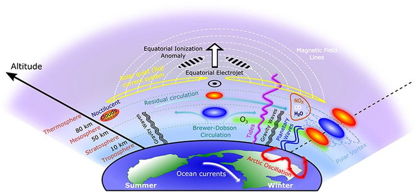
FIG. 27-2. Schematic of the BDC as the combined effect of residual circulation and mixing in
the stratosphere and mesosphere. The thick white arrows depict the TEM mass streamfunction
as representation of the residual circulation, whereas the wavy orange arrows indicate two-way
mixing processes. Both circulation and mixing are mainly induced by wave activity on different
scales (planetary to gravity waves). The thick green lines represent stratospheric transport and
mixing barriers. Note that the vertical scale compresses the mesosphere above 50 km. [Figure is
courtesy of U. Schmidt.]
Another major theoretical development in the 1990s of the BDC and its driving mechanisms, and most
was the introduction of the concept of ‘‘mean age of air’’ notably its projected response to climate change. An
(Hall and Plumb 1994), which is based on the mean important gap in current knowledge about the BDC
transit time for air to reach a particular location in the is a comprehensive understanding of how wave driving
stratosphere after entry from the troposphere. This of the stratosphere has changed in response to climate
single metric combines the effects of the transport by the change. Changes in the troposphere could influence
BDC with those of the mixing by eddies (Kida 1983). the strength of the upward propagating waves, while
Climate model projections suggest a shorter transit time changes in the background state of the stratosphere
in the future (i.e., ‘‘younger’’ age of air) as a result of will change the way in which the waves propagate (e.g.,
climate change (Butchart and Scaife 2001). Apart from Bell et al. 2010), and how much of their momentum
in the subtropical lower stratosphere, where this can will get deposited in the flow (e.g., Lubis et al. 2018).
only result from a strengthened BDC, the younger age Critical-layer control on Rossby wave breaking has
generally indicates both the possibility of a strengthen- been invoked as a possible mechanism (Shepherd and
ing of the BDC and/or weaker mixing or recirculation of McLandress 2011). However, changes in wave-driving
the stratospheric air between the tropics and mid- in response to climate change are still uncertain, es-
latitudes (Garny et al. 2014). pecially the relative changes between wave-forcing
In recent years a synergy of these developments has due to planetary waves (zonal wavenumbers 1–3),
led to a more quantitative, dynamically based analysis which drive the deep branch of the BDC (Plumb 2002);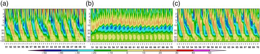
CHAPTER 27                                     BALDWIN ET AL.                                                      27.7

synoptic-scale waves (zonal wavenumbers 4 and higher),      3. Middle atmosphere dynamics theory
which drive the shallow branch of the BDC; and
                                                              The thermodynamic state and the flow in the middle
gravity waves, which are important in the mesosphere
                                                            atmosphere are governed by dynamics as well as the
and above (section 6) and the QBO (section 7). Fur-
                                                            complex balance between radiation and photochemical
ther detailed studies will be required to shed more
                                                            processes that heat and cool the atmosphere. Heating is
light onto this.
                                                            dominated by absorption of solar radiation by ozone in
   A changing BDC will affect many aspects of the
                                                            the stratosphere and molecular oxygen in the thermo-
stratosphere, though arguably the most significant im-
                                                            sphere, while cooling is dominated by infrared emission,
pacts will be observed in the recovery of stratospheric
                                                            mostly by carbon dioxide (CO2) (e.g., Murgatroyd and
ozone (e.g., Shepherd 2008; Bekki et al. 2011; Dhomse
                                                            Goody 1958). Large deviations of the temperature field
et al. 2018), in changes in the lifetimes of ozone-
                                                            from the state of radiative equilibrium are caused by
depleting substances and some greenhouse gases (e.g.,
                                                            adiabatic heating and cooling processes, which are driven
Butchart and Scaife 2001), in the exchange of mass be-
                                                            by waves (Leovy 1964). The three principal theoretical
tween the stratosphere and the troposphere with impli-
                                                            paradigms that are applied to middle atmosphere dy-
cations for tropospheric ozone (e.g., Zeng and Pyle 2003;
                                                            namics are as follows: 1) wave propagation, 2) wave
Meul et al. 2018), and in levels of ultraviolet (UV) ra-
                                                            mean–flow interaction, and 3) the mean overturning cir-
diation reaching Earth’s surface (e.g., Hegglin and
                                                            culation response to radiative forcing and wave driving.
Shepherd 2009; Meul et al. 2016).
   As noted above, stratosphere-resolving GCMs and             The most important wave modes for middle atmo-
CCMs consistently project a strengthening of the BDC        sphere theory are atmospheric gravity waves (see sec-
in response to greenhouse gas–induced climate change        tion 6), whose restoring force is buoyancy due to gravity
(Rind et al. 1990; Butchart and Scaife 2001; Butchart       and stable stratification, and Rossby waves (see section 5),
et al. 2006; Garcia and Randel 2008; Li et al. 2008;        for which a combination of differential planetary rotation
Calvo and Garcia 2009; McLandress and Shepherd              and stratification provides the restoring force. On spatial
2009; Butchart et al. 2010a,b; Okamoto et al. 2011;         scales larger than a few hundred kilometers, gravity waves
Bunzel and Schmidt 2013; Oberländer et al. 2013).           are modified by Earth’s rotation and are known as
Depending on the greenhouse gas scenario considered,        inertia–gravity waves. A third type of wave is the atmo-
these projections translate into a 2.0%–3.2% decade21       spheric Kelvin wave, which is analogous to coastal Kelvin
increase in the net upwelling mass flux in the tropical     waves in the ocean. It exists in the atmosphere because of
lower stratosphere (which is typically chosen as a          the change in sign of the Coriolis parameter at the
measure of the overall strength of the BDC). On the         equator, which provides geostrophic balance in the lat-
other hand, actual changes in the circulation can only      itudinal direction, but its restoring force is otherwise
be inferred indirectly from observations of long-lived      buoyancy (Holton and Lindzen 1968).
trace gases and, as yet, there is no conclusive obser-         Wave propagation theory tells us how the waves
vational evidence that the BDC is either speeding up or     propagate and where they are likely to get absorbed, or
slowing down (Engel et al. 2009; Diallo et al. 2012;        if they will get reflected back to their source region.
Seviour et al. 2012; Stiller et al. 2012). However, the     Wave propagation differs among the different wave
latest evidence suggests that the BDC changes have a        types, but their interaction with the mean flow shares
vertical structure, with a strengthening of the shallow     some common features (e.g., Eliassen and Palm 1961),
branch in the lower to midstratosphere (Bönisch et al.      namely, that under steady, nondissipative conditions,
2011) and a weakening of the deep branch above that,        the waves conserve wave pseudomomentum flux. The
thus reconciling at least some of the discrepancies         pseudomomentum indicates the strength of the drag on
(Hegglin et al. 2014).                                      the flow when the waves are dissipated. Thus, waves
   Finally, modeling evidence is now emerging that a        affect the flow nonlocally, by essentially transporting
changing BDC may have a significant role in the dy-         momentum from their source region to where they dis-
namical coupling between the stratosphere and tropo-        sipate. This dissipation exerts a drag on the mean flow,
sphere with implications for surface climate and weather    which modifies it both directly and indirectly by driving
(e.g., Baldwin et al. 2007a; Karpechko and Manzini          an overturning circulation in response (see section 2).
2012; Scaife et al. 2012). Therefore, it appears that the      The theory of atmospheric gravity waves can be
influences of the BDC and its response to climate           traced back to the works of eminent eighteenth-century
change may not be solely confined to the stratosphere       scientists such as Euler, Lagrange, Laplace, and Newton
but are almost certainly omnipresent throughout Earth’s     on water waves, but the crucial role of buoyancy in
atmosphere.                                                 atmospheric gravity waves began with the works of
27.8                                         METEOROLOGICAL MONOGRAPHS                                          VOLUME 59

Väisälä (1925) and Brunt (1927), who independently de-          Rossby (1939). The equation for Rossby wave propa-
rived the frequency of oscillation of an air parcel displaced   gation from the troposphere into the stratosphere was
vertically in a stably stratified dry atmosphere, which now     first derived by Charney and Drazin (1961) and later
bears their name, the Brunt–Väisälä frequency,                  extended to include latitudinal propagation by
                     vffiffiffiffiffiffiffiffiffiffiffiffiffiffiffiffiffiffiffiffiffiffiffiffiffiffiffi               Dickinson (1968) and Matsuno (1970). It indicates that
                     u                       !
                     u g ›T g                                   Rossby waves can only propagate to the stratosphere if
                  N 5t              1             ,   (27-1)    the zonal flow is westerly and below a certain critical
                      T ›z cp
                                                                value, and if the wavenumber is small. This explained
                                                                why stratospheric Rossby waves are planetary scale and
where g is the acceleration due to gravity, T is tempera-
                                                                only found in winter (Charney and Drazin 1961).
ture, z is altitude, and cp is the specific heat at constant
                                                                Moreover, the equations also indicate the existence of
pressure. This buoyancy restoring force acting on slanted
                                                                two kinds of surfaces that block wave propagation—
displacements gives rise to gravity waves that propagate
                                                                critical surfaces that lead to wave absorption (Eliassen
both vertically and horizontally (see Lindzen 1973). The
                                                                and Palm 1961; Matsuno 1971) and turning surfaces that
dissipation of gravity waves results from several processes,
                                                                reflect the waves (Sato 1974; Harnik and Lindzen 2001).
namely, radiative damping (Fels 1984), gravity wave
                                                                   The dispersion relation for atmospheric Rossby waves,
breaking (Lindzen 1981), and other nonlinear wave–wave
                                                                using the quasigeostrophic (QG) approximation, is
processes (see the review by Fritts and Alexander 2003).
All these processes are strongest near critical levels—                                   ›q0
where the horizontal phase speed of the wave equals the                                       k
                                                                                          ›y
mean flow speed (e.g., Booker and Bretherton 1967;                            v
                                                                              ^ 52                   ,              (27-3)
                                                                                           f2     f2
Lindzen 1981). Gravity wave drag is especially strong in                          k2h 1 m2 2 2 2 2
                                                                                          N     4N H
the mesosphere and is responsible for reversing the me-
ridional temperature gradient (summer pole is coldest)          where f 5 2V sinf is the Coriolis parameter; V being the
and forcing the strong meridional summer-to-winter pole         rotation frequency of Earth; f is latitude; ›q0 /›y is the
circulation (Lindzen 1981).                                     meridional gradient of mean flow quasigeostrophic po-
   Many of the gravity waves have horizontal and vertical       tential vorticity (QGPV), which has a planetary compo-
scales that are too small to be resolved in climate models      nent b 5 ›f/›y 5 (2V cosf)/a and a contribution from the
and must be parameterized (e.g., Lindzen 1981; McFarlane        meridional and vertical curvature of the zonal-mean zonal
1987; Hines 1997; Alexander and Dunkerton 1999; Warner          wind (see, e.g., appendix of Harnik and Lindzen 2001); y is
and McIntyre 2001). The dispersion relation for atmo-           the latitudinal distance coordinate; and a is Earth’s mean
spheric gravity waves, neglecting the effects of                radius, and we have simplified the equations by assuming
Earth’s rotation and compressibility for simplicity, is         QG dynamics and a zonal-mean flow (typically assumed
                                                                for Rossby waves), with constant N2 and an exponentialy
                                 N 2 k2h                        decreasing pressure with scale height H.
                   ^2 5
                   v                              ,   (27-2)
                                            1                      The linear theory for atmospheric gravity waves can
                          k2h 1 m2 1
                                           4H 2                 be modified easily to include the local effects of plane-
                                                                tary rotation leading to a generalization of the disper-
where kh is horizontal wavenumber satisfying
                                                                sion relation (27-2) for ‘‘inertia–gravity waves’’ (e.g.,
k2h 5 k2 1 l2 , with k, l being the zonal and meridional
                                                                Holton and Hakim 2013, 153–154). Including the effects
wavenumbers, respectively; v    ^ is the intrinsic wave fre-
                                                                of Earth’s rotation near the equator leads to an-
quency: v ^ 5 v 2 ku0 2 ly 0 , with v being the wave fre-
                                                                other class of wave modes denoted ‘‘equatorial waves’’
quency and u0 and y 0 the zonal and meridional mean
                                                                (Matsuno 1966). The gravitational influence of the sun
flow velocities, respectively; m is the vertical wave-
                                                                and moon, as well as the sun’s heating effects, gives rise
number; and H is the pressure-scale height. The vertical
                                                                to the atmospheric tides, waves with frequencies related
group velocity, ›v/›m, is oppositely directed relative to
                                                                to the astronomical frequencies of the solar and lunar
the vertical phase velocity in the frame of reference
                                                                days [see Chapman and Lindzen (1970) and section 4].
relative to the mean wind. Assuming a small mean-wind
                                                                   The following fundamental relationships for atmo-
Doppler shift, one can easily derive the direction of the
                                                                spheric wave mean–flow interactions have their origins
vertical group velocity, which is the sense of wave energy
                                                                in Eliassen and Palm (1961). For adiabatic flow with f 5 0,
propagation (see, e.g., Fritts and Alexander 2003).
                                                                no wave transience, and u0 2 c 6¼ 0,
   Conservation of potential vorticity (PV) gives rise to
atmospheric planetary waves, also known as Rossby
waves after C.-G. Rossby, who introduced them in                                p0 w0 5 2r0 (u0 2 c)u0 w0 ,         (27-4)
CHAPTER 27 BALDWIN ET AL. 27.9
FIG. 27-3. (a) Climatological January zonally averaged zonal-mean wind as a function of pressure altitude and latitude (positive in-
dicates north) for 1980–99 from the ERA-40 reanalysis dataset. (b) As in (a), but from a GISS model with no gravity wave parameter-
ization. (c) As in (b), from the same GISS model with a gravity wave parameterization included. [Panels (a) and (b) are from Fig. 1 and
(c) is from Fig. 6 of Geller et al. (2011).]
› nonacceleration theorem appears to be a negative re-
(r u0 w0 ) 5 0, (27-5)
›z 0 sult, it is important in that it identifies those factors that
give rise to wave mean–flow interactions.
where p and w are the pressure and vertical velocity, re-
SSWs are a spectacular example of wave–mean flow
spectively; r is the basic state density; u0 is the basic state
interaction in the middle atmosphere involving Rossby
flow, taken here to be the zonal-mean wind; the primes
waves, first successfully modeled by Matsuno (1971) and
indicate wave quantities; c is the wave phase velocity; and
described in detail in section 5 below. Why SSWs occur
overbars denote averages over wave phase. Equation (27-4)
during specific winters and not others is not yet clear,
indicates that if u0 . c, an upward (group) propagating
however, it has been shown that downward reflection of
wave (upward energy flux p0 w0 . 0) will have negative
waves dominates the daily variability during most of the
vertical flux of horizontal momentum (r0 u0 w0 ); that is to
winters which lack SSWs (Perlwitz and Harnik 2003).
say, the waves will tend to decelerate the mean flow to-
Many of the interannual differences can be rationalized
ward the wave phase velocity in the presence of dissipa-
as arising from the different effects which SSWs (wave
tive effects. It also indicates that waves cannot propagate
absorption) and wave reflection have on the mean flow
vertically through critical levels.
deceleration (Perlwitz and Harnik 2004), on the result-
Equation (27-5) implies that in the absence of wave ing overturning circulation (Shaw and Perlwitz 2014),
transience and critical levels and diabatic effects, there is and correspondingly on poleward ozone transport and
no interaction between waves and the mean flow. The concentrations (Lubis et al. 2017).
Eliassen–Palm relationships in Eqs. (27-4) and (27-5) Examples of wave–mean flow interaction involving
have been generalized by Andrews and McIntyre gravity waves are shown in Figs. 27-3 and 27-4, using re-
(1978a,b,c) and Boyd (1976) and have led to the TEM sults from some NASA Goddard Institute for Space
(see section 1) formulation of the dynamics, which re- Studies (GISS) models. Note that the upper-stratospheric
lates the Eulerian zonal-mean fields to the approximate winds are excessive in Fig. 27-3b, and are much more
Lagrangian overturning meridional-vertical circulation, excessive in the winter NH than in the summer SH. The
considering wave-induced Stokes drift effects. The TEM Fig. 27-3c winds, while not agreeing perfectly with those
equations are discussed in the general circulation in Fig. 27-3a, are much more realistic in both hemi-
chapter of this monograph (Held 2019). spheres. Comparing Figs. 27-3b and 27-3c, we see that
The Eliassen–Palm relations imply the well-known gravity waves play a major role in making the upper-
nonacceleration theorem; that is to say, for steady waves stratospheric winds more realistic in Fig. 27-3c in the
with no dissipation and no critical levels, waves propa- winter hemisphere, while they play a lesser role in the
gate through the mean flow without leading to acceler- summer hemisphere.
ations or decelerations. An important counterpart to Another aspect of the importance of the wave–mean
this is the nontransport theorem, which states that under flow interactions is shown in Fig. 27-4. The QBO (de-
the conditions for nonacceleration, no net transport by scribed in more detail in section 7) is a quasiperiodic
the waves occurs for chemical species that have lifetimes reversal in the equatorial mean zonal wind in the lower
much longer than the dynamic time scales. While the stratosphere with a mean period of about 28 months.27.10 METEOROLOGICAL MONOGRAPHS VOLUME 59
FIG. 27-4. Mean zonal wind in m s21 at pressure altitudes of 100–1 hPa averaged between 48S and 48N (a) for the years 1991–2010 from
ERA-40, (b) for the years 1951–70 from a GISS model with an equatorial parameterized gravity wave momentum flux of 0.5 mPa, and
(c) for the GISS model as in (b), but with an equatorial parameterized gravity wave momentum flux of 3.0 mPa. [From Fig. 1 of Geller et al.
(2016).]
The first successful explanation for the QBO was given zonal winds, and this can act as a transport barrier. It was
by LH68, in terms of wave–mean flow interaction. It pointed out by McIntyre and Palmer (1983) that plan-
involves a constant wave flux of easterly and westerly etary wave breaking gives rise to the mixing of chemical
momentum at a bottom boundary, notionally taken to constituents and PV at midlatitudes, and while this tends
be the tropopause. When the mean wind is greater than to reduce latitudinal PV gradients where the mixing
zero (u0 . 0), there is preferential absorption of westerly occurs, in the region referred to as the ‘‘surf zone’’
momentum at lower levels, and the easterly momentum (McIntyre and Palmer 1984), it also serves to strengthen
flux penetrates to high levels, giving rise to easterly (u0 , 0) the gradients at the subtropical and polar edges of the
wind at high levels. The easterly and westerly winds surf zone. One consequence of this is the sharpening of
descend until easterly winds prevail at lower levels. the large PV gradients at the edge of the vortex. The
Then, the situation repeats giving rise to the QBO [see very large PV gradients at the equatorward edge of the
Plumb (1977) for a schematic illustration of this pro- SH polar vortex that acts as a transport barrier has been
cess]. Figure 27-4a shows an example of the QBO os- referred to as a ‘‘containment vessel,’’ where the air
cillation in the mean zonal wind averaged between 48S inside that vortex is largely isolated from the lower-
and 48N from the ERA-40 reanalysis. Figures 27-4b and latitude air. This was a crucial aspect of explaining the
27-4c show the same plot from a GISS model with a Antarctic ozone hole (see Solomon et al. 1986). Erosion
gravity wave parameterization, with gravity wave mo- of the large PV gradients at the edge of the NH polar
mentum flux at 100 hPa at the equator equal to 0.5 and vortex was also suggested by McIntyre (1982) to be
3.0 mPa, respectively. crucial in setting the conditions for SSWs. Finally, ex-
PV is another concept that is extremely useful in amination of transport processes in the vicinity of the
middle atmosphere dynamics, and is defined as large PV gradients at the equatorward edge of the surf
zone, which can also impede transport across the sub-
PV 5 2g(›u/›p)(zu 1 f ) , tropics, has led to the concept of the tropical ‘‘leaky
pipe’’ (see Plumb 1996).
where g is gravity, u is potential temperature, p is pres- There are many more theoretical concepts in middle
sure, zu is relative vorticity evaluated along isentropic atmosphere dynamics. Because of space limitation, we
surfaces, and f is the Coriolis parameter. During the have concentrated on the wave–mean flow interaction as
1980s, advances were made in our understanding of the main paradigm in the field. Many of the theoretical
stratospheric dynamics by applying ‘‘PV thinking’’ approaches outlined above have been quasi-linear, in
(Hoskins et al. 1985). PV has large gradients between the sense that the waves interact with the mean flow, but
the troposphere and stratosphere near the tropopause. not with each other. This is an unrealistic assumption,
In fact, this has led to defining the ‘‘dynamical tropo- but such models have served the field well as a template
pause’’ in terms of a given PV value in the extratropics for understanding middle atmosphere dynamics.
(e.g., see Hoskins et al. 1985). See section 8 for a more
general discussion of the tropopause.
4. Atmospheric thermal tides
PV generally increases poleward, largely due to f in-
creasing, but in winter there is usually a particularly Atmospheric thermal tides are global-scale, periodic
large PV gradient at the edge of the winter polar vortex, oscillations that are excited mainly by absorption of
due to large variations in the horizontal shear of the solar radiation by ozone and water vapor, and by latentCHAPTER 27 BALDWIN ET AL. 27.11 heating due to tropical deep convection. The thermal (Lindzen 1981). These processes can make a substantial tides were first documented through their signature in contribution to the momentum and thermodynamics surface pressure. These ‘‘barometric tides’’ are re- budgets of the thermosphere (e.g., Becker 2017). markable in that the semidiurnal oscillation has much Much recent work on atmospheric thermal tides has greater amplitude than the diurnal, even though so- focused on their behavior in the range of altitude from lar heating is obviously dominated by its diurnal the tropopause (10–15 km) to the lower thermosphere component. The paradox was noted explicitly by Kelvin (;150 km), as discussed in the recent review article by (Thomson 1882), who hypothesized that the larger am- Oberheide et al. (2015). England (2012) has reviewed plitude of the semidiurnal tide relative to the diurnal the tides at even higher altitudes, in the ionosphere. could be explained by the existence of a ‘‘free,’’ or res- Sassi et al. (2013) used a global model extending to onant, solution of Laplace’s tidal equation with period 500 km to study the migrating and nonmigrating tides near 12 h. in the thermosphere and showed that the diurnal tide The effort to substantiate Kelvin’s hypothesis led to undergoes a striking change in structure in the lower systematic exploration of Laplace’s tidal equation as thermosphere, where the upward-propagating (1, 1) applied to Earth’s stratified atmosphere. These studies, mode disappears due to dissipation by molecular together with the increasing ability to observe temper- diffusion. The (1, 1) designation refers to the westward- ature and winds above the tropopause using radiosondes propagating, wavenumber 1, first mode of the inertia– and—beginning in the late 1940s—rocketsondes, shaped gravity wave manifold (see Chapman and Lindzen our current understanding of the tides throughout 1970), which is the main component of the upward- Earth’s atmosphere. It was found that heating due to propagating diurnal tide. Above ;120 km, the (1, 1) absorption of solar radiation by ozone in the strato- mode is replaced by a latitudinally broad, nonpropagating sphere and water vapor in the troposphere were the external mode, which is forced by in situ extreme UV leading sources of excitation (e.g., Siebert 1961; Butler solar heating. and Small 1963). Kelvin’s resonance hypothesis was Nonmigrating or, more properly, non-sun-synchronous eventually discarded, and the unexpectedly small am- tides have been documented recently in observations of plitude of the diurnal surface pressure tide was shown to the mesosphere and lower thermosphere. These are arise from the propagation characteristics of the tidal oscillations whose periods are harmonics of the solar day ‘‘modes’’ that are solutions to the tidal equations. Spe- but do not propagate westward following the sun. They cifically, the diurnal component of ozone heating in the arise from diurnal but spatially fixed forcing, associated stratosphere projects most strongly on modes that are principally with the diurnal cycle of deep convective nonpropagating, or ‘‘trapped,’’ whereas the semidiurnal heating in the troposphere (Lindzen 1978; Hamilton component can propagate to the surface (Kato 1966; 1981; Forbes et al. 1997). Along these lines, Gurubaran Lindzen 1966, 1967). The history of this work, together et al. (2005) and Pedatella and Liu (2012) have docu- with the development of the mathematical theory of the mented an apparent modulation of tidal amplitudes by tides, is summarized in Chapman and Lindzen’s (1970) El Niño–Southern Oscillation (ENSO), which is a monograph on the subject. principal source of interannual variability in tropical The introduction of satellite-borne observing systems convection. Several nonmigrating tides have been ob- in the late 1970s enormously enhanced the ability to served (Talaat and Lieberman 1999, 2010; Forbes and document the global behavior of the tides from the Wu 2006; Li et al. 2015), including an eastward- troposphere to very high altitudes in the ionosphere. At propagating wavenumber-3 diurnal oscillation (DE3), the same time, rapidly increasing computational capa- which features prominently in satellite observations of bilities allowed numerical solution of the tidal equations the mesosphere and lower thermosphere. The structure in atmospheric global models and detailed comparisons of DE3 is shown in Fig. 27-5, which is constructed from between numerical predictions and observations. The observations made by the Sounding of the Atmosphere amplitude of nondissipating waves in a stratified atmo- Using Broadband Emission Radiometry (SABER) in- sphere grows with altitude, z, as exp(z/2H), where H is frared radiometer (Russell et al. 1999) using squared the scale height, such that the temperature and wind coherence analysis, as detailed by Garcia et al. (2005). perturbations associated with the tides become very The role of DE3 in coupling the lower thermosphere to large in the mesosphere. At still higher altitudes, in the the ionosphere has been demonstrated by Immel et al. thermosphere, growth of these waves ceases as they are (2006), who documented a link between longitudinal damped by molecular diffusion. Amplitude growth can variability in ionospheric density in the F region (250– also be limited by dissipation due to wave ‘‘breaking’’ if 400 km) and the amplitude of nonmigrating diurnal the tides become dynamically or convectively unstable tides. The link operates mainly via tidal modulation of
27.12                                    METEOROLOGICAL MONOGRAPHS                                                          VOLUME 59

                                                                        FIG. 27-6. Amplitude variation of the diurnal migrating tide
   FIG. 27-5. Mean amplitude and phase structure of the diurnal,     (DW1) over the period 2002–17 as seen in SABER temperature
eastward-propagating tide of wavenumber 3 (DE3) in the range of      data. A prominent semiannual variation is evident above 10 scale
altitude 7–16 scale heights (;49–112 km) obtained via coherence      heights (;70 km) together with substantial interannual modula-
analysis of SABER data over the period 2002–17 (see Garcia et al.    tion. Both the semiannual and interannual variability appear to be
2005). The base point for the coherence analysis is denoted by the   related to the variability of the tropical zonal-mean zonal wind at
red cross; results are shown only where the squared coherence        lower altitudes (cf. Fig. 27-7).
statistic is significant at the 95% level. As can be seen from the
phase structure, the DE3 tide is predominantly equatorially anti-    term, [ f 2 (›u0/›y)], near the equator, where f is small
symmetric below 14 scale heights (;98 km), and symmetric above
that level. This suggests that forcing of DE3 projects onto both
                                                                     and comparable to ›u0/›y. Burrage et al. (1995),
antisymmetric inertia–gravity and symmetric Kelvin modes. The        Lieberman (1997), and Vincent et al. (1998) have re-
amplitude is large (8 K) in the lower thermosphere.                  ported interannual variability in the amplitude of the
                                                                     diurnal tide, which is apparently related to the strato-
                                                                     spheric QBO. This behavior has been reproduced in a
the electric field in the E region (100–150 km), which in            numerical model by McLandress (2002b), who con-
turn couples to the F region (Hagan et al. 2007; Xiong               cluded that the mechanism responsible for the semi-
and Lühr 2013). This discovery established a link be-                annual modulation of the diurnal tide also causes the
tween ‘‘space weather’’ and the tropospheric weather                 quasi-biennial modulation. Smith et al. (2017) have
(tropical convection) that excites DE3. England et al.               shown recently that temperature data from the SABER
(2010) have also explored the impact of tides on the                 and Microwave Limb Sounder (MLS) satellite in-
ionosphere and further illustrated the coupling between              struments can be used to estimate the zonal-mean zonal
tides in the lower thermosphere and electron density in              winds in the tropics (Fig. 27-8). Comparison of Figs. 27-6
the ionosphere.                                                      and 27-7 shows the relationship between the diurnal tide
   Tides in the middle atmosphere display marked sea-                in the MLT and the tropical winds. It may be possible to
sonal and interannual variability. Radar observations                use such data, derived from a common source, to eluci-
(Vincent et al. 1998) show that the amplitude of the                 date further the relationship between tidal amplitudes
diurnal (1, 1) migrating tide has a prominent semiannual             and tropical mean zonal wind variations.
variation in the mesosphere and lower thermosphere                      Despite these advances, it is apparent that accurate
(MLT). This variability is also seen in satellite obser-             simulation of the tides in comprehensive numerical
vations (e.g., Hays et al. 1994; Burrage et al. 1995)                models remains a challenge. For example, Davis et al.
Semiannual and quasi-biennial modulations in tidal                   (2013) used meteor radar data at Ascension Island to
amplitudes are clearly displayed in data obtained                    investigate the seasonal variability of the diurnal and
from the SABER instrument, as shown in Fig. 27-6.                    semidiurnal tides and noted that two leading ‘‘high-top’’
McLandress (2002a) used a linear mechanistic model                   models produce results that are not in general agreement
to attribute the semiannual variation to changes in                  with observations. A possible reason for these discrep-
the horizontal shear of the background zonal-mean                    ancies is that simulation of the tropical wind oscillations,
wind u0, and argued that this influences the tide mainly             the QBO and the semiannual oscillation (SAO), is still
through its contribution to the barotropic vorticity                 unsatisfactory in many comprehensive numerical models.
You can also read