BOUNDING GLOBAL AEROSOL RADIATIVE FORCING OF CLIMATE CHANGE - MPG.PURE

REVIEW ARTICLE Bounding Global Aerosol Radiative Forcing
10.1029/2019RG000660
 of Climate Change
Key Points:
• An assessment of multiple lines of N. Bellouin1 , J. Quaas2 , E. Gryspeerdt3 , S. Kinne4 , P. Stier5 , D. Watson-Parris5 ,
 evidence supported by a conceptual O. Boucher6 , K. S. Carslaw7 , M. Christensen5 , A.-L. Daniau8 , J.-L. Dufresne9 ,
 model provides ranges for aerosol
 radiative forcing of climate change
 G. Feingold10 , S. Fiedler4,28 , P. Forster11 , A. Gettelman12 , J. M. Haywood13,14 ,
• Aerosol effective radiative forcing U. Lohmann15 , F. Malavelle13 , T. Mauritsen16 , D. T. McCoy7 , G. Myhre17 ,
 is assessed to be between -1.6 J. Mülmenstädt2 , D. Neubauer15 , A. Possner18,19 , M. Rugenstein4 , Y. Sato20,21 ,
 and -0.6 W m−2 at the 16–84%
 confidence level
 M. Schulz22 , S. E. Schwartz23 , O. Sourdeval2,24 , T. Storelvmo25 , V. Toll1,26 ,
• Although key uncertainties remain, D. Winker27 , and B. Stevens4
 new ways of using observations
 provide stronger constraints for 1 Department of Meteorology, University of Reading, Reading, UK, 2 Institute for Meteorology, Universität Leipzig,
 models Leipzig, Germany, 3 Space and Atmospheric Physics Group, Imperial College London, London, UK, 4 Max Planck
 Institute for Meteorology, Hamburg, Germany, 5 Atmospheric, Oceanic and Planetary Physics, Department of Physics,
Correspondence to: University of Oxford, Oxford, UK, 6 Institut Pierre-Simon Laplace, Sorbonne Université/CNRS, Paris, France, 7 School of
N. Bellouin, Earth and Environment, University of Leeds, Leeds, UK, 8 EPOC, UMR 5805, CNRS-Université de Bordeaux, Pessac,
n.bellouin@reading.ac.uk France, 9 Laboratoire de Météorologie Dynamique/IPSL, CNRS, Sorbonne Université, Ecole Normale Supérieure, PSL
 Research University, Ecole Polytechnique, Paris, France, 10 NOAA ESRL Chemical Sciences Division, Boulder, CO, USA,
 11 Priestley International Centre for Climate, University of Leeds, Leeds, UK, 12 National Center for Atmospheric
Citation:
Bellouin, N., Quaas, J., Gryspeerdt, Research, Boulder, CO, USA, 13 CEMPS, University of Exeter, Exeter, UK, 14 UK Met Office Hadley Centre, Exeter, UK,
E., Kinne, S., Stier, P., Watson-Parris, 15 Institute for Atmospheric and Climate Science, ETH Zürich, Zürich, Switzerland, 16 Department of Meteorology,
D., et al. (2020). Bounding global
 Stockholm University, Stockholm, Sweden, 17 Center for International Climate and Environmental Research-Oslo
aerosol radiative forcing of climate
change. Reviews of Geophysics, 58, (CICERO), Oslo, Norway, 18 Department of Global Ecology, Carnegie Institution for Science, Stanford, CA, USA, 19 Now
e2019RG000660. https://doi.org/10. at Institute for Atmospheric and Environmental Sciences, Goethe University, Frankfurt, Germany, 20 Department of
1029/2019RG000660 Applied Energy, Graduate School of Engineering, Nagoya University, Nagoya, Japan, 21 Now at Faculty of Science,
 Department of Earth and Planetary Sciences, Hokkaido University, Sapporo, Japan, 22 Climate Modelling and Air
Received 16 MAY 2019 Pollution Section, Research and Development Department, Norwegian Meteorological Institute, Oslo, Norway,
 23 Brookhaven National Laboratory Environmental and Climate Sciences Department, Upton, NY, USA, 24 Laboratoire
Accepted 3 OCT 2019
Accepted article online 1 NOV 2019 d'Optique Atmosphérique, Université de Lille, Villeneuve d'Ascq, France, 25 Department of Geosciences, University of
 Oslo, Oslo, Norway, 26 Now at Institute of Physics, University of Tartu, Tartu, Estonia, 27 NASA Langley Research Center,
 Hampton, VA, USA, 28 Now at Institut für Geophysik und Meteorologie,Universität zu Köln, Köln, Germany

 Abstract Aerosols interact with radiation and clouds. Substantial progress made over the past 40 years
 in observing, understanding, and modeling these processes helped quantify the imbalance in the Earth's
 radiation budget caused by anthropogenic aerosols, called aerosol radiative forcing, but uncertainties
 remain large. This review provides a new range of aerosol radiative forcing over the industrial era based
 on multiple, traceable, and arguable lines of evidence, including modeling approaches, theoretical
 considerations, and observations. Improved understanding of aerosol absorption and the causes of trends
 in surface radiative fluxes constrain the forcing from aerosol-radiation interactions. A robust theoretical
 foundation and convincing evidence constrain the forcing caused by aerosol-driven increases in liquid
 cloud droplet number concentration. However, the influence of anthropogenic aerosols on cloud liquid
 water content and cloud fraction is less clear, and the influence on mixed-phase and ice clouds remains
 poorly constrained. Observed changes in surface temperature and radiative fluxes provide additional
 constraints. These multiple lines of evidence lead to a 68% confidence interval for the total aerosol effective
 radiative forcing of -1.6 to -0.6 W m−2 , or -2.0 to -0.4 W m−2 with a 90% likelihood. Those intervals are
 of similar width to the last Intergovernmental Panel on Climate Change assessment but shifted toward
 more negative values. The uncertainty will narrow in the future by continuing to critically combine
©2019. The Authors.
 multiple lines of evidence, especially those addressing industrial-era changes in aerosol sources and
This is an open access article under aerosol effects on liquid cloud amount and on ice clouds.
the terms of the Creative Commons
Attribution License, which permits
use, distribution and reproduction in
 Plain Language Summary Human activities emit into the atmosphere small liquid and solid
any medium, provided the original particles called aerosols. Those aerosols change the energy budget of the Earth and trigger climate changes,
work is properly cited. by scattering and absorbing solar and terrestrial radiation and playing important roles in the formation of

BELLOUIN ET AL. 1 of 45

Reviews of Geophysics 10.1029/2019RG000660

 cloud droplets and ice crystals. But because aerosols are much more varied in their chemical composition
 and much more heterogeneous in their spatial and temporal distributions than greenhouse gases, their
 perturbation to the energy budget, called radiative forcing, is much more uncertain. This review uses
 traceable and arguable lines of evidence, supported by aerosol studies published over the past 40 years,
 to quantify that uncertainty. It finds that there are two chances out of three that aerosols from human
 activities have increased scattering and absorption of solar radiation by 14% to 29% and cloud droplet
 number concentration by 5 to 17% in the period 2005–2015 compared to the year 1850. Those increases
 exert a radiative forcing that offsets between a fifth and a half of the radiative forcing by greenhouse
 gases. The degree to which human activities affect natural aerosol levels, and the response of clouds, and
 especially ice clouds, to aerosol perturbations remain particularly uncertain.

 1. Introduction
 At steady state and averaged over a suitably long period, the heat content in the Earth system, defined here
 as the ocean, the atmosphere, the land surface, and the cryosphere, remains constant because incoming
 radiative fluxes balance their outgoing counterparts. Perturbations to the radiative balance force the state of
 the system to change. Those perturbations can be natural, for example, due to variations in the astronomical
 parameters of the Earth, a change in solar radiative output or injections of gases and aerosol particles by
 volcanic eruptions. Perturbations can also be due to human activities, which change the composition of the
 atmosphere.
 A key objective of Earth system sciences is to understand historical changes in the energy budget of the Earth
 over the industrial period (Myhre et al., 2017) and how they translate into changes in the state variables
 of the atmosphere, land, and ocean; to attribute observed temperature change since preindustrial times to
 specific perturbations (Jones et al., 2016); and to predict the impact of projected emission changes on the cli-
 mate system. From that understanding climate scientists can derive estimates of the amount of committed
 warming that can be expected from past emissions (Pincus & Mauritsen, 2017; Schwartz, 2018), estimates
 of net carbon dioxide emissions that would be consistent with maintaining the increase in global mean sur-
 face temperature below agreed targets (Allen et al., 2018), or the efficacy of climate engineering to possibly
 mitigate against climate changes in the future (Kravitz et al., 2015).
 A sustained radiative perturbation imposed on the climate system initially exerts a transient imbalance in the
 energy budget, which is called a radiative forcing (RF; denoted as  ; Figure 1a). The system then responds
 by eventually reaching a new steady state whereby its heat content once again remains fairly constant. The
 equilibrium change in global mean surface temperature ΔTs , in K, is given by

 ΔTs =  (1)

 where  is the global mean RF, in W m−2 , and is the climate sensitivity parameter that quantifies the
 combined effect of feedbacks, in K (W m−2 )−1 (Ramanathan, 1975). For multiple reasons, including lack of
 knowledge of and the long response time of Ts to RF (Forster, 2016; Knutti et al., 2017; Schwartz, 2012), it
 has become customary to compare the strengths of different perturbations by their RFs rather than by the
 changes in Ts that ultimately ensue.
 Temperatures in the stratosphere, a region of the atmosphere which is largely uncoupled from the
 troposphere-land-ocean system below, respond on a timescale of months, adjusting the magnitude and in the
 case of ozone perturbations even the sign of the initial RF (Figure 1b) (Hansen et al., 1997). This adjusted RF
 is defined by the 5th Assessment Report (AR5) of the Intergovernmental Panel on Climate Change (IPCC)
 (Myhre, Shindell, et al., 2013) as the change in net downward radiative flux at the tropopause, holding tropo-
 spheric state variables fixed at their unperturbed state but allowing for stratospheric temperatures to adjust
 to radiative equilibrium. This definition is adopted by this review.
 In addition to exerting a RF, changes in atmospheric composition affect other global mean quantities, such
 as temperature, moisture, surface radiative and heat fluxes, and wind fields, as well as their spatiotemporal
 patterns. Some of these responses occur on timescales much faster than the adjustment timescales of ocean
 surface temperatures. These responses are called rapid adjustments and occur independently of surface
 temperature change (Hansen et al., 2005; Shine et al., 2003). Rapid adjustment mechanisms can augment

BELLOUIN ET AL. 2 of 45

Reviews of Geophysics 10.1029/2019RG000660

 Figure 1. (a) Instantaneous radiative forcing: A perturbation is applied, but the vertical profiles of temperature
 (solid line) and moisture remain unperturbed. (b) Stratosphere-adjusted radiative forcing: Stratospheric temperatures
 respond (transition from dashed to solid line). (c) Effective radiative forcing: The perturbation also triggers rapid
 adjustments in the troposphere, but surface temperatures have not yet responded. (d) The system returns to radiative
 balance by a change in surface temperature.

 or offset the initial RF by a sizable fraction, because they involve changes to the radiative properties of the
 atmosphere, including clouds, and/or the surface, which all contribute substantially to the Earth's energy
 budget. Consequently, effective radiative forcing (ERF; denoted  ; Figure 1c), which is the sum of RF and
 the associated rapid adjustments, is a better predictor of ΔTs than RF (Figure 1d). Sherwood et al. (2015)
 make a pedagogical presentation of the concept of rapid adjustments that was used in IPCC AR5 (Boucher
 et al., 2013; Myhre, Shindell, et al., 2013). This review also adopts the definition of ERF introduced in the
 IPCC AR5 (Boucher et al., 2013; Myhre, Shindell, et al., 2013), which is the change in net top-of-atmosphere
 downward radiative flux that includes adjustments of temperatures, water vapor, and clouds throughout the
 atmosphere, including the stratosphere, but with sea surface temperature maintained fixed. In addition to
 its influence on global temperature change, ERF is also an efficient predictor of changes in globally averaged
 precipitation rate (Andrews et al., 2010). Those changes arise from a balance between radiative changes
 within the atmosphere and changes in the latent and sensible heat fluxes at the surface (Richardson et al.,
 2016). Accounting for rapid adjustments when quantifying radiative changes is essential to obtain the full
 response of precipitation.
 RF can be induced in multiple ways: changes in atmospheric composition, both in the gaseous and partic-
 ulate phases, induced by volcanic or anthropogenic emissions; changes in surface albedo; and variations in
 solar irradiance. An estimated full range of anthropogenic aerosol RF based on an elicitation of 24 experts
 of −0.3 W m−2 to −2.1 W m−2 at the 90% confidence level was presented by Morgan et al. (2006). Individ-
 ual experts, however, allowed for the possibility of much more negative, but also the possibility even of net
 positive, RF. A similar degree of uncertainty has been reflected in an evolving series of IPCC assessment
 reports (Table 1), where best estimates and uncertainty ranges of aerosol RF are also based at least partly

 Table 1
 Best Estimates and Uncertainty Ranges of Radiative Forcing of Aerosol-Radiation and Aerosol-Cloud Interactions, and
 Total Aerosol Radiative Forcing, in W m−2 , as Given by Successive Assessment Reports of the IPCC
 Assessment Forcing Aerosol-radiation Aerosol-cloud Total
 report period interactions interactions
 2 (Schimel et al., 1996) 1750–1993 −0.50 (−1.00 to −0.25) N/A (−1.5 to 0.0) N/A
 3 (Penner et al., 2001) 1750–1998 N/A N/A (−2 to 0.0) N/A
 4 (Forster et al., 2007) 1750–2005 −0.50 (−0.90 to −0.10) −0.70 (−1.80 to −0.30) −1.3 (−2.2 to −0.5)
 5 Boucher et al. (2013) 1750–2011 −0.45 (−0.95 to +0.05) −0.45 (−1.2 to 0.0) −0.9 (−1.9 to −0.1)
 Note. Uncertainty ranges are given at the 90% confidence level. The First Assessment Report did not have the scientific
 understanding needed to quantify aerosol radiative forcing, although they noted that it was potentially substantial.
 All values are for radiative forcing, except for the Fifth Assessment Report, which are for effective radiative forcing.
 Adapted from Table 8.6 of (Myhre, Shindell, et al., 2013).

BELLOUIN ET AL. 3 of 45

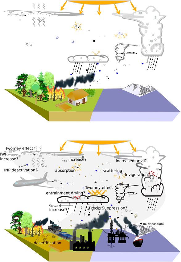
Reviews of Geophysics 10.1029/2019RG000660

 on expert judgment. Since RFs are additive within the forcing-response paradigm, the uncertainty attached
 to the aerosol ERF translates to the entire anthropogenic ERF (Schwartz & Andreae, 1996). Recognition of
 this fact has motivated a tremendous effort, now lasting several decades, to better understand how aerosols
 influence radiation, clouds, and ultimately the large-scale trajectory of the climate system, involving field
 measurements, laboratory studies, and modeling from microphysical to global scales (e.g., Ghan & Schwartz,
 2007; Kulmala et al., 2011; Seinfeld et al., 2016).
 In spring 2018, under the auspices of the World Climate Research Programme's Grand Science Challenge
 on Clouds, Circulation and Climate Sensitivity, 36 experts gathered at Schloss Ringberg, in the mountains of
 Southern Germany, to take a fresh and comprehensive look at the present state of understanding of aerosol
 ERF and identify prospects for progress on some of the most pressing open questions, thereby drawing the
 outlines for this review. The participants at that workshop expressed a wide range of views regarding the
 mechanisms and magnitudes of aerosol influences on the Earth's energy budget. This review represents a
 synthesis of these views and the underlying evidence.
 This review is structured as follows. Section 2 reviews the physical mechanisms by which anthropogenic
 aerosols exert an RF of climate and sets the scope of this review. Section 3 presents a conceptual model of
 globally averaged aerosol ERF and the different lines of evidence used to quantify the uncertainty bounds in
 the terms of that conceptual model. Section 4 quantifies changes in aerosol amounts between preindustrial
 and present-day conditions. Sections 5 and 6 review current knowledge of aerosol interactions with radiation
 and clouds, respectively, to propose bounds for their RF, while sections 7 and 8, respectively, do the same for
 their rapid adjustments. Section 9 reviews the knowledge, and gaps thereof, in aerosol-cloud interactions
 in ice clouds. Section 10 reviews estimates of aerosol ERF based on the response of the climate system over
 the last century. Finally, section 11 brings all lines of evidence together to bound total global aerosol ERF
 and outlines open questions and research directions that could further contribute to narrow uncertainty or
 reduce the likelihood of surprises.

 2. Mechanisms, Scope, and Terminology
 2.1. Aerosol RF Mechanisms
 The term “atmospheric aerosol” denotes a suspension of microscopic and submicroscopic particles in air.
 These particles may be primary, meaning emitted directly in the liquid or solid phase, or secondary, meaning
 that they are produced in the atmosphere from gaseous precursors. In both cases, sources may be natural, for
 example, sand storms, sea spray, volcanoes, natural wildfires, and biogenic emissions, or result from human
 activities, like construction and cement production, agriculture, and combustion of biomass and fossil fuels
 (Hoesly et al., 2018). Once in the atmosphere, aerosols undergo microphysical (e.g., coagulation and con-
 densation) and chemical (e.g., oxidation) transformation and are transported with the atmospheric flow.
 Tropospheric aerosols, the aerosols of main concern here, remain in the atmosphere for days to weeks (e.g.,
 Kristiansen et al., 2012). Those relatively short residence times, compared to greenhouse gases, are caused
 by efficient removal processes, either by direct deposition to the surface by sedimentation, diffusion, or tur-
 bulence or by scavenging by and into cloud droplets and ice crystals, and subsequent precipitation. As a
 consequence of these relatively rapid removal processes together with spatially heterogeneous distribution
 of sources, tropospheric aerosols are highly nonuniform spatially and temporally: A mean residence time
 of approximately 5 days results in typical transport distances of about 2000 km. In consequence, aerosols
 are concentrated in and downwind of source regions such as cities and industrialized regions. In contrast,
 aerosols introduced into the stratosphere, for example, by explosive volcanic eruptions, may have residence
 times of several months to a few years because of slow particle sedimentation velocities and secondary
 aerosol production.
 Aerosols modify the Earth's radiative budget directly through scattering and absorption of radiation, denoted
 here aerosol radiative interaction, ari, and indirectly by modifying the microphysical properties of clouds,
 affecting their reflectivity and persistence, denoted here aerosol-cloud interactions, aci (Figure 2). Aerosols
 may also affect the reflectivity of the surface, as absorbing aerosol deposited on snow-covered surfaces may
 decrease their reflectivity. As a result of these processes, anthropogenic emissions of aerosols and their
 gaseous precursors have over the Anthropocene exerted an ERF, which is thought to have been strength-
 ening over time for much of the industrial period, but is locally and instantaneously highly variable. All of
 this heterogeneity combines to make the aerosol ERF challenging to quantify, not just locally, but also in the
 global and annual mean.

BELLOUIN ET AL. 4 of 45

Reviews of Geophysics 10.1029/2019RG000660

 Figure 2. Simplified representation of the impact of anthropogenic aerosol emissions on the Earth system in (a) the
 preindustrial and (b) the present-day atmosphere. A schematic representation of known processes relevant for the
 effective radiative forcing of anthropogenic aerosol is summarized for present-day conditions in panel (b), but the same
 processes were active, with different strengths, in preindustrial conditions. Processes where the impact on the effective
 radiative forcing remains qualitatively uncertain are followed by a question mark. liquid and ice denote liquid and ice
 cloud fractions, respectively. LWP and IWP stand for liquid and ice water path, respectively. INP stands for ice
 nucleating particle.

BELLOUIN ET AL. 5 of 45

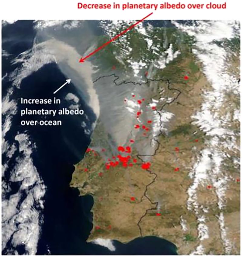
Reviews of Geophysics 10.1029/2019RG000660

 Aerosol-radiation interactions are readily discerned by human observers
 as smoke, haze, and dust (see box). As early as the fifteenth century,
 Leonardo da Vinci in instructions on how to paint a battle scene noted
 that the distribution of light in a mineral dust and biomass burning plume
 was such that “from the side whence the light comes this mixture of air
 and smoke and dust will seem far brighter than on the opposite side” (Paris
 Manuscript A, circa 1492), a manifestation of the angular distribution of
 light scattering that must be accurately represented in calculation of the
 RF. Volcanic aerosols and their impact on sunsets have also influenced
 a wide range of artists as shown by Zerefos et al. (2014). In this context
 the possibility that anthropogenic and volcanic aerosols decrease atmo-
 spheric transmittance of solar radiation globally was therefore considered
 relatively early in climate change studies (e.g., McCormick & Ludwig,
 1967; Mitchell, 1971).
 Improvements in the physical understanding of atmospheric scatter-
 ing and absorption, combined with a good constraint on ocean surface
 reflectance, allowed Haywood et al. (1999) to show that ari was needed to
 explain satellite-retrieved top-of-atmosphere shortwave radiative fluxes
 under cloud-free conditions. Aerosol contributions to outgoing short-
 wave radiative fluxes can exceed 100 W m−2 in some cases, as estimated
Figure 3. True-color satellite image taken by the Moderate Resolution for example, by Haywood et al. (2003) from aircraft measurements of a
Imaging Spectroradiometer (MODIS) showing a plume of smoke from
 mineral dust plume over the ocean. In addition to these direct effects
forest fires in Portugal on 3 August 2003. Fires are shown by the red spots;
the smoke plume appears in gray. From Haywood (2015). of scattering and absorption, rapid adjustments to ari, originally called
 semidirect effects, were postulated by Grassl (1975), then again more
 recently from global modeling (Hansen et al., 1997), and observations
 made during the Indian Ocean Experiment (INDOEX) field campaign (Ackerman et al., 2000). Those adjust-
 ments stem from changes in the distribution of atmospheric radiative fluxes and heating rates induced by
 the aerosols, especially light-absorbing aerosols, which then modify surface radiative and heat fluxes, tem-
 perature and water vapor profiles, atmospheric stability, and the conditions for cloud formation (Stjern et al.,
 2017). Correlations between satellite retrievals of aerosol, clouds, and planetary albedo consistent with the
 expected signature of semidirect effects have been reported, for example, over the subtropical South Atlantic
 Ocean (Wilcox, 2012) and North Atlantic marine stratocumulus decks (Amiri-Farahani et al., 2017).

 “Impact of absorption on aerosol-radiation interactions”
 Aerosol particles scatter and absorb solar (also called shortwave) and terrestrial (or longwave)
 radiation, hereafter denoted aerosol-radiation interaction (ari). The efficiency at which they do so
 depends on the wavelength of the radiation, the distribution of particle sizes, their shapes, and on
 their refractive index, which is determined by their chemical composition and mixing state (Hansen
 & Travis, 1974). For each particle, both scattering and absorption contribute to the extinction of radi-
 ation, and the single-scattering albedo (SSA), denoted 0 , quantifies the contribution of scattering
 to total extinction:
 sca
 0 = (2)
 sca + abs

 where sca and abs are the scattering and absorption cross sections, respectively, in units of area.
 This key quantity can be likewise defined for a population of aerosol particles.
 Locally and seen from the top of the atmosphere, aerosol particles can both increase or decrease
 the amount of radiation reflected to space, depending on the contrast between the brightness
 of the aerosols and that of the underlying surface. Bright (scattering) aerosols increase the local
 albedo when over dark surfaces but have less of an impact when over brighter surfaces. Conversely,
 dark (absorbing) aerosols decrease the albedo over bright surfaces but have less of an impact over

BELLOUIN ET AL. 6 of 45

Reviews of Geophysics 10.1029/2019RG000660

 darker surfaces. This effect is clearly demonstrated by the satellite image shown in Figure3 show-
 ing biomass burning aerosol over the Iberian Peninsula. The absorbing smoke plume brightens the
 image when located over dark land and ocean surfaces but darkens it when overlying the bright
 cloud to the northwest.

 Mathematically, that change in sign of the aerosol-radiation interactions means that there exists a
 SSA, named critical SSA (Chýlek & Coakley, 1974) and denoted 0crit , where aerosols have the same
 brightness as the underlying surface and thus exert no radiative perturbation in spite of interacting
 with radiation. Haywood and Shine (1995) have expressed 0crit as a function of the surface albedo,
 s , and the mean fraction of radiation up-scattered to space by the aerosols, , as follows:
 2 s
 0crit = (3)
 (1 − s )2 + 2 s
 Quantities in this equation are integrated and weighted over the solar spectrum. In practice, the
 critical SSA ranges from 0.7 and 0.8 over land surfaces (e.g., Gonzi et al., 2007) and is up to 0.9 over
 clouds (Costantino, 2012). Most aerosols from natural and human sources have a SSA larger than
 0.9 and therefore typically increase reflection of radiation to space, but aerosols from agricultural
 and forest fires are often more strongly absorbing, and decrease reflection of radiation when located
 above clouds (e.g., Leahy et al., 2007; Zuidema et al., 2016). The point where the radiative effect of
 aerosol-radiation interactions switches sign from negative to positive has alternatively been char-
 acterized as a critical surface albedo (King et al., 1999) or a critical cloud fraction (Chand et al.,
 2009).

 Clouds affect aerosol populations. They act as a source of aerosol mass, because heterogeneous chemistry
 converts precursor gases into low-volatile or nonvolatile chemical components of aerosol, and as a sink of
 aerosols because precipitation is the main pathway for removing aerosols from the atmosphere. But aerosols
 also affect clouds.
 Aerosol-cloud interactions are based, for liquid clouds, on the role aerosol particles play as cloud conden-
 sation nuclei (CCN), first identified by Aitken (1880) and then described thermodynamically by Köhler
 (1936). An anthropogenically driven increase in CCN concentrations therefore leads to more cloud droplets.
 Conover (1966), Hobbs et al. (1970) and Twomey (1974) presented observational evidence for increases in
 CCN resulting in increases in droplet number. More numerous droplets present an increased scattering cross
 section leading to an increase of the albedo of the cloud when liquid water path (LWP) is held constant. In
 radiative transfer the particle size is often measured by a droplet effective radius, re , rather than the droplet
 number concentration, Nd , so it is often stated that an increase in Nd , for a given cloud liquid water content,
 implies a decrease in re . This was the original formulation by Twomey (1977). Ship tracks, the quasi-linear
 features of enhanced cloud albedo along the track of ships (Conover, 1966), are commonly cited as evidence
 for that cloud brightening.
 Ice clouds also contribute to aci. This is the case when ice crystals form via homogeneous freezing of water
 droplets or aqueous aerosol particles, and because some aerosols serve as ice nucleating particles (INPs)
 (DeMott et al., 1997). Changes to liquid droplets may also have later implications for the ice phase in
 mixed-phase clouds (Coopman et al., 2018; Norgren et al., 2018). Observations of higher concentrations of
 smaller ice crystals in cirrus clouds polluted by aircraft exhaust were first made by Ström and Ohlsson (1998)
 and Zhao et al. (2018) found similar correlations in satellite retrievals, although seasonal variations in water
 vapor overwhelm the aerosol signature. Vergara-Temprado, Miltenberger, et al. (2018) have shown by com-
 paring a global model to satellite retrievals of radiative fluxes that INP concentrations can strongly alter the
 reflectivity of shallow mixed-phase clouds. However, evidence for a Twomey effect acting on ice clouds is
 far from being as strong as for liquid clouds.
 The list of rapid adjustments associated with aci is long. Because of different processes, adjustments in liq-
 uid clouds, in mixed-phase, and ice clouds are usually considered separately. But even among clouds of

BELLOUIN ET AL. 7 of 45

Reviews of Geophysics 10.1029/2019RG000660

 the same phase, differences in cloud dynamics or environmental conditions may influence the sign of the
 adjustment. Adjustments in liquid clouds have been hypothesized through aerosol increases driving delays
 in precipitation rates (Albrecht, 1989) and increases in cloud thickness (Pincus & Baker, 1994) that would
 manifest themselves as increases in cloud LWP or changes in cloud fraction (CF). Altered droplet size distri-
 butions also affect entrainment mixing of clouds with environmental air, possibly reducing LWP (Ackerman
 et al., 2004; Small et al., 2009). The latter adjustments might reduce the increase in cloud albedo (Stevens &
 Feingold, 2009). Adjustments in mixed phase and ice clouds stem from different mechanisms. Responses of
 these clouds to aerosols include more frequent glaciation of supercooled water because of preferential freez-
 ing onto increased INP (Lohmann, 2002), deactivation of INP because of changes in aerosol mixing state
 (Girard et al., 2004; Hoose et al., 2008; Storelvmo et al., 2008), changes in precipitation and consequently
 cloud water path and cloud reflectivity (Vergara-Temprado, Miltenberger, et al., 2018), invigoration of con-
 vection from suppression of precipitation and latent heat release (Khain et al., 2001; Koren et al., 2005), and
 increase in lightning occurrence in deep convective clouds (Thornton et al., 2017).
 Aerosols may also exert an RF after their removal from the atmosphere. Aerosol-surface interactions refer
 to changes in albedo from the deposition of absorbing aerosols on to bright—for example, snow- and
 ice-covered—surfaces. Initially hypothesized by Bloch (1965) to explain past changes in sea level, the impact
 of aerosols on snow albedo was quantified by Warren and Wiscombe (1980), who showed that including
 in-snow aerosol absorption in a radiative transfer model better fits albedo measurements made in the Arctic
 and Antarctica. Rapid adjustments to aerosol-surface interactions involve changes in snow grain size and
 the timing of melting of the snow pack (Flanner et al., 2007). Since such effects are relevant only in confined
 regions, they are not assessed in detail in this review.
 Compared to greenhouse gases, aerosols exhibit much more variable chemical compositions and much
 shorter atmospheric residence times, but much greater forcing per unit mass from interaction with radia-
 tion. For ari, aerosol scattering and absorption cross sections depend on the wavelength of the radiation and
 the physical and chemical properties of the aerosol (see box). The sign and strength of the RF due to ari,
 RFari, is modulated further by environmental factors, including incident radiation, relative humidity, and
 the albedo of the underlying ocean, land surface or cloud (See Figure 3). For aci, the ability of aerosol parti-
 cles to serve as CCN or INPs depends on the number concentration, size distribution, solubility, shape, and
 surface chemical properties of the particles. In addition, cloud type or cloud regime, that is, discrimination
 between cumuliform and stratiform clouds, as well as clouds in different altitudes (WMO, 2017) is a strong
 determinant of the complex responses of cloud processes to an aerosol-driven increase in drop number,
 and those cloud processes may be more important and uncertain for aci than aerosol processes (Gettelman,
 2015). Even if all of these issues could be addressed accurately, uncertainty would remain due to uncertainty
 in the reference state (Carslaw et al., 2013), increasingly so the further back in time one adopts a baseline.
 2.2. Scope and Definitions
 The scope of this review is globally averaged aerosol ERF because the concept of ERF is mostly relevant to
 the understanding of climate change in a global sense. Consequently, ERF from aerosol-surface interactions
 due to deposition of absorbing aerosols on to snow and ice is not considered here because it comes primarily
 from local areas within high latitude regions or high mountain ranges and does not contribute much to the
 globally averaged ERF (Jiao et al., 2014). The strong regional variations in aerosol distributions and ERF may
 matter for determining impacts of aerosol ERF on several aspects of the Earth system (e.g. Bollasina et al.,
 2011; Chung and Soden, 2017; Kasoar et al., 2018), but those considerations are also not addressed in this
 review. Both RF and ERF are measured in W m−2 and cover both the solar (shortwave, SW) and terrestrial
 (longwave, LW) parts of the electromagnetic spectrum.
 Although this review adopts the IPCC definitions of RF and ERF (Myhre, Shindell, et al., 2013), it differs
 from previous IPCC practices in two ways. First, the reference year is chosen to be 1850 instead of 1750.
 Although 1750 represents a preindustrial state when fossil fuel combustion emissions were negligible, there
 is no evidence for 1750 being special from an aerosol point of view, as agricultural fires occurred well before
 that. In addition, 1850 matches the start of most surface temperature records and also the start of the his-
 torical climate simulations of the Coupled Model Intercomparison Project (CMIP; Eyring et al., 2016). This
 match is important because having coincidence in the starting year is beneficial to comparing the change
 in forcing with the change in temperature. The difference in RF between the two reference years is smaller
 than 0.1 W m−2 (Myhre, Shindell, et al., 2013; Carslaw et al., 2017) because industrialization was still in its

BELLOUIN ET AL. 8 of 45

Reviews of Geophysics 10.1029/2019RG000660

 early stages in 1850. The ERF between the years 1750 and 1850 has been estimated at −0.2 W m−2 by the
 IPCC AR5 (Myhre, Shindell, et al., 2013) but it could have been as weak as −0.028 W m−2 according to sim-
 ulations using more recent emissions (Lund et al. 2019). For present day, (Myhre, Shindell, et al., 2013) used
 2011 but this review is slightly more generic so present day refers here to average aerosol concentrations over
 the period 2005–2015. Second, this review will not attempt to bound aerosol RF mechanisms for which lines
 of evidence remain fragile, which increases the possibility that the bounds derived here are too conservative.
 Consequently, uncertainty ranges are given in this review as 16–84% confidence intervals (68% likelihood
 of being in the ranges given, equivalent to ±1- for a normal distribution) instead of the 5–95% confidence
 interval (90% likelihood of being in the range) generally considered in IPCC Assessment Reports. The main
 uncertainty ranges are however translated to 5–95% confidence intervals in section 11 and Table 5 to make
 comparison easier.
 To quantify the confidence intervals for RF and ERF, this review will need to combine the 16–84% confidence
 intervals obtained for different quantities. To do so, each 16–84% confidence interval is first expanded to a full
 interval (0–100% confidence) by assuming that probabilities are uniformly distributed within the interval,
 that is, by extending the range by a factor 100/68. Full intervals are then sampled randomly 10 million
 times in a Monte Carlo framework similar to that of Boucher and Haywood (2001), with the difference that
 they applied the uniform distribution approach to a case where the terms are added rather than multiplied.
 Finally, the resulting intervals are reported with 16–84% confidence.

 3. Conceptual Model and Lines and Evidence
 3.1. Conceptual Model
 The net radiative flux, R, at the top of the atmosphere is the difference between the globally and annually
 averaged absorbed insolation (SW), R↓SW (1 − ), and outgoing terrestrial (LW) irradiance, R↑LW :

 R = R↓SW (1 − ) − R↑ LW ≈ 0 (4)

 where the near equality of the two denotes a state of stationarity. The albedo, , the fraction of the insolation
 that is scattered back to space, depends on the properties of the atmosphere, the surface, and the angle of
 illumination. Aerosol perturbations primarily affect , in which context their effect stems from changes in
 the column-integrated extinction coefficient of the aerosol, called aerosol optical depth (AOD) and denoted
 a , and in cloud droplet number concentrations, Nd . a is usually dominated by scattering, but some sub-
 components of the aerosol are also absorbing in the SW or LW parts of the electromagnetic spectrum and
 contribute to the net irradiance absorbed by the atmosphere, Ratm . Similarly to extinction, aerosol absorption
 is usually quantified by the aerosol absorption optical depth, abs . Nd depends on another subcomponent of
 the aerosol, namely, the number of hygroscopic aerosol particles that serve as CCN. Anthropogenic aerosol,
 through its forcing and consequent rapid adjustments of clouds as well as through its direct interaction with
 terrestrial radiation, may also contribute to changes in R↑LW . Aerosol-induced changes in ice clouds may
 also influence R. Changes in surface properties are assumed small relative to the magnitude of the other
 components in the global annual mean.
 Adopting this description leads to the expectation that a change in the amount or properties of aerosol
 influences the net irradiance and thus exerts an RF,  , as follows
 R R ||
  = ΔR = Δ a + Δ ln Nd (5)
 a ln Nd ||,
 where Δ a and Δ ln Nd denote the perturbation in global AOD and relative perturbation in cloud droplet
 number concentration, respectively, taken here as the difference between 1850 and an average year between
 2005 and 2015, hereafter called for convenience “preindustrial” and “present-day,” respectively.  denotes
 the cloud LWP and  the cloud fraction, and the second partial derivative therefore excludes changes in those
 quantities, following Twomey (1974). Equation (5) is valid for a given point in space and time. Perturbations
 in a and Nd are not independent, but the two terms in equation (5) assume a decoupling between radiative
 changes originating in the clear part of the atmosphere from those originating in the cloudy part of the
 atmosphere. However, it should be noted that this assumption is not equivalent to decoupling changes in
 clear-sky and cloudy-sky radiative fluxes.
 Rapid adjustments are added to  to obtain the ERF,  . For ari, this consists of a term describing changes to
 Ratm driven by changes in a . Changes in Ratm then impact R, including R↑LW , and cloud amount. For aci, this

BELLOUIN ET AL. 9 of 45

Reviews of Geophysics 10.1029/2019RG000660

 modifies the sensitivity of R to changes in Nd to allow for changes in  and  , in cloud top temperature and
 hence R↑LW , and in ice clouds. The inclusion of rapid adjustments is represented mathematically by moving
 from partial to total derivatives:
 R dR dRatm dR
  = Δ a + Δ a + Δ ln Nd . (6)
 a dRatm d a d ln Nd

 The literature does not decompose rapid adjustments of a or abs on cloud properties into adjustments of
  and  separately (Bond et al., 2013; Koch & Del Genio, 2010), so these rapid adjustments are included
 in the overall sensitivity of Ratm to a through the second term on the right-hand side of equation (6). In
 contrast, such decomposition is commonly performed for aci (Chen et al., 2014; Gryspeerdt, Goren, et al.,
 2019; Mülmenstädt et al., 2019; Quaas et al., 2008; Sekiguchi et al., 2003). For a given point in space and time,
 the sensitivity of R to changes in Nd , d lndRN , neglecting the changes in ice clouds and in cloud top temperature,
 d
 consists of the change in response solely due to changes in Nd with everything else constant—relevant for
 the RF due to aci, RFaci (equation (5))—and the radiative impact of the adjustments. The sensitivity is best
 expressed as logarithmic in Nd , because most cloud processes are sensitive to a relative, rather than absolute,
 change in Nd (Carslaw et al., 2013, see also Eq. 17). This approach is also supported by satellite data analyses
 (e.g., Kaufman & Koren, 2006; Nakajima et al., 2001; Sekiguchi et al., 2003). The total response of R to relative
 perturbations in Nd can therefore be expanded as
 dR R || R d R d
 ≈ + + = SN + S,N + S,N . (7)
 d ln Nd ln Nd ||,  d ln Nd  d ln Nd

 The first and third terms are restricted to cloudy regions. The last step defines the denotation of the three
 terms as radiative sensitivities, SN , S,N , and S,N .
 In some cases, usually under idealized conditions, the sensitivities expressed by the partial derivatives
 in equations (6) and (7) can be calculated theoretically or inferred observationally. For instance, under
 clear skies R∕ a can be calculated locally and averaged over different scenes to get a global sensitivity
 of top-of-atmosphere net radiation to changes in a . To relate this global sensitivity to the global, all-sky
 response requires also accounting for situations where there is little sensitivity. For instance, over a suffi-
 ciently bright background, like a snow-covered surface or a cloud, increasing the clear-sky scattering will
 have no appreciable effect on , irrespective of the magnitude of the aerosol perturbation. Likewise, over a
 dark surface increasing aerosol absorption has little effect on (see box).
 This assessment targets the global, annual mean aerosol ERF so there is a need to integrate equations (6)
 and (7), which are valid at a given location in space and time, globally and over periods of time long enough
 to eliminate variability from changes in the weather. In particular, the aci sensitivities defined in equation 7
 require averaging globally over the different cloud regimes that experience changes in Nd . Weighting factors
 are introduced to account for those spatial and temporal dependencies, following Steven (2015). Although
 these weighting factors are related to cloud amount, clouds span a distribution of optical depths and their
 optical depth differently mediates the extent to which they mask ari or express aci. So the weighting factors
 are effective cloud fractions, denoted c, and the effective clear-sky fraction need not be the complement of the
 effective cloudy-sky fraction. The introduction of the weighting factors allows for an attractive framework to
 quantify the aerosol RFs and their uncertainties, at the expense of having to quantify the uncertainties of the
 weighting factors themselves. These uncertainties may be larger than the uncertainty on CF but arguments
 can be made to estimate them.
 Effective cloud fractions c , cN , c , and c are therefore introduced for each term in equation 8. They are
 formally defined, and quantified from the literature, in sections 5, 6, and 8, respectively. Consequently, the
 individual terms in equations (6) and (7) are parameterized as a product of the change in the global aerosol
 or cloud state, idealized sensitivities (S) and those weighting factors (c). Applying this approach to equations
 (6) and (7) yields the following formula for :
 [ ]
 dR dRatm [ ]
  = Δ a S clear (1 − c ) + S cloudy c + + Δ ln Nd SN cN + S,N c + S,N c (8)
 dRatm d a

 The term representing  ari has been decomposed into cloud-free and cloudy contributions to properly
 account for the masking or enhancement of ari by clouds, as discussed above. The sensitivity S clear is defined

BELLOUIN ET AL. 10 of 45

Reviews of Geophysics 10.1029/2019RG000660

Table 2
Mathematical Definitions and Descriptions of the Variables of Equations (8), (15), and (24)
Section Mathematical definition Description
4 aPD Present day (2005–2015) a
4 Δ a = aPD − aPI Change in a between present day (2005–2015)
 and preindustrial (1850)
4 Δ ln a = Δ a ∕ aPD Relative change in a over the industrial era
6 Δ ln Nd = ΔNd ∕Nd Relative change in Nd over the industrial era
 Aerosol-radiation interactions
5 S clear = Rclear ∕ a Sensitivity of R to changes in a in clear (cloud-free) sky
 cloudy
5 S = Rcloudy ∕ a Sensitivity of R to changes in a in cloudy-sky
 ⟨ c Δ a ⟩
5 c = ⟨ c Δ a ⟩
 Effective cloud fraction for RFari
7 dR∕dRatm Sensitivity of R to changes in
 atmospheric absorption
7 dRatm ∕d a Sensitivity of atmospheric absorption to
 changes in a
 Aerosol-cloud interactions
 ln Nd
6 ln N−ln = ln a
 Sensitivity of Nd to changes in a
 R ||
6 SN = ln Nd ||
 Sensitivity of R to changes in Nd at constant  and 
 ,
 R↓SW ⟩
 Δ a
 ⟨liq c (1− c ) ln N−ln a
 a
6 cN = Δ a ↓
 Effective cloud fraction for RFaci
 ⟨ c ⟩⟨ ⟩⟨
 ( c ) ln N−ln a a
 1− ⟩⟨RSW
 ⟩
 ln 
8 ln −ln N = ln Nd
 Sensitivity of  to changes in Nd
 R d
8 S,N =  d ln Nd
 Sensitivity of R to changes in 
 mediated by changes in Nd
 Δ a ↓
 ⟨liq c (1− c ) ln −ln Nd ln N −ln a R ⟩
 a SW
8 c = d
 Effective cloud fraction for rapid adjustments in 
 ⟨ a ⟩⟨R↓SW ⟩
 Δ 
 ⟨ c (1− c )⟩ ⟨ ln −ln N ⟩
 ⟨ ln N −ln a ⟩
 d d a
 
8 −ln N = ln N Sensitivity of  to changes in Nd
 d
 R d
8 S,N =  d ln Nd
 Sensitivity of R to changes in 
 mediated by changed in Nd
 R↓SW ⟩
 Δ a
 ⟨(1−ice ) ( c − clear ) −ln N ln N−ln a a
8 c = Effective cloud fraction for rapid adjustments
 ⟨ a ⟩⟨R↓SW ⟩
 Δ 
 ⟨( c − clear )⟩⟨ −ln N ⟩ ⟨ ln N−ln a ⟩
 a

 in cloud fraction
Note. The first column gives the number of the section where the uncertainty range for each variable is assessed. a and c are the aerosol and cloud optical
depths, respectively. Nd is the cloud droplet number concentration.  is the liquid cloud water path.  is the cloud fraction, and liq and ice are the liquid
and ice cloud fractions, respectively. R is the sum of shortwave and longwave radiation at the top of the atmosphere, Ratm is the radiation absorbed in the
atmosphere, and R↓SW is the downwelling shortwave radiation at cloud top. c and clear are the cloud and cloud-free albedos, respectively. Angle brackets denote
global-area-weighted temporal averaging.

 R cloudy
 cloudy R
 as clear . Similarly, S is defined as . Sensitivities that are a product of two partial derivatives, as
 a a
 defined by equation (7), are denoted by a double subscript. For reference, Table 2 summarizes the definitions
 of the variables used in equation (8).
 An important and long standing objection to the approach embodied by equation (8) is that because aerosol
 perturbations are large and local, their effects are nonlinear, and cannot be related to perturbations of the
 global aerosol state. However, such effects can be incorporated into the weighting factors. For instance, when
 applying the interpretive framework of equation (8) to the output from models that spatially and temporally
 resolve ari, it becomes possible to assess the extent to which differences arise from differences in how they
 represent the intrinsic sensitivity, S , the magnitude of the perturbation, Δ a , or the way in which local
 effects are scaled up globally, as measured by c . To the extent that nonlinearities are important—and often
 for global averages of very nonlinear local processes they are not—it means that the weighting factors, c,
 may be situation dependent, and their interpretation may be nontrivial.

BELLOUIN ET AL. 11 of 45

Reviews of Geophysics 10.1029/2019RG000660

 The ari term of equation (8) has been assumed linear in Δ a . This assumption is justified by a series of
 arguments that starts at the source of the aerosol. For primary aerosols, aerosol number concentrations are
 linear in the emission rate. For secondary aerosols, linear relationships between emissions of gaseous pre-
 cursor and RFari have been found at the global scale, including for precursors like dimethyl-sulfide (Rap
 et al., 2013). The aerosol population undergoes fast microphysical aging processes right after emission or
 nucleation (Jacobson & Seinfeld, 2004), changing its size, composition, and mixing state. These microphys-
 ical processes grow anthropogenic nanoparticles into sizes comparable to the wavelength of the radiation,
 where aerosols interact efficiently with radiation. Preexisting aerosol particles act both as condensational
 sinks of gas-phase precursors and as seeds to efficiently grow semivolatile aerosol precursors to ari-relevant
 sizes. The overall scaling of secondary aerosol number concentrations from nucleation therefore depends on
 relative emission rates of primary and secondary aerosol precursors. Estimates from global microphysical
 aerosol models that include aerosol nucleation, condensation and coagulation confirm nonlinear responses
 to the coemission of primary carbonaceous aerosols and sulfur dioxide (SO2 , a precursor to sulfate aerosols),
 in particular near aerosol source regions (Stier et al., 2006). However, these deviations do not exceed 30%
 locally for accumulation mode number concentrations and 15% for a , sufficiently small to be assumed lin-
 ear in the global mean context of this review. Further, ari scales fairly linearly with Δ a for a given SSA
 (Boucher et al., 1998). The SSA of the aerosol population, which moderates the top-of-atmosphere ERF (see
 box), depends on the composition of aerosol sources, specifically the fraction of anthropogenic absorbing
 aerosols and notably black carbon (BC; also called soot (Bond et al., 2013)) aerosols. These factors affect the
 clear-sky albedo sensitivity S and the atmospheric absorption efficiency dRatm ∕d a .
 Finally, equation (8) may require an additional term to represent changes in ice cloud properties in response
 to changes in ice crystal number, but scientific understanding is not there yet to support a quantitative
 assessment of that term, as discussed in section 9.
 3.2. Lines of Evidence
 From a historical point of view, process-oriented studies at the relevant aerosol and cloud scales are the foun-
 dation of the conceptual thinking of aerosol RF. Observational and modeling tools have led to investigations
 that have helped refine process understanding and generate further lines of investigation with increasingly
 sharp tools.
 For the purpose of this review, lines of evidence are grouped into three categories: estimation of sensitivities
 of radiation and clouds to aerosol changes; estimation of large-scale changes in the aerosol and cloud states
 over the industrial era; and inferences from observed changes in the overall Earth system.
 3.2.1. Estimation of Sensitivities
 There are several methods with the potential to estimate sensitivities of radiation and clouds to aerosol
 changes:
 • In situ observations using ground-based and airborne instruments;
 • Remote sensing observations from ground-based networks, airborne, and satellite platforms;
 • Process-based modeling at small scales using cloud-resolving models or large eddy models.
 Airborne measurements that combine cloud droplet size, droplet number, liquid water and cloud-reflected
 radiance (Brenguier et al., 2003; Werner et al., 2014), and high-quality ground-based measurements, for
 example, from supersites, have provided strong, quantitative evidence for aerosol effects on cloud micro-
 physics (Brenguier et al., 2003; Feingold et al., 2003; Garrett et al., 2003; Kim et al., 2003; Twomey &
 Warner, 1967). However, translating those effects to the radiative response and deriving sensitivities remains
 a challenge. For example, negative correlations between droplet size and aerosol concentration support the
 underlying theory proposed by Twomey (1977) but confound droplet size responses to aerosol with cloud
 water responses to the aerosol and its associated meteorology (e.g. Brenguier et al., 2003) and thus make it
 difficult to unravel the net radiative response. Quantification of sensitivities has proven to be contingent on
 a variety of factors, including choice of instrument, retrieval accuracy (Sena et al., 2016), aggregation scale
 (McComiskey & Feingold, 2012), and cloud regime. Drizzle is also a confounding factor that obscures the
 relationships, reducing droplet number and increasing droplet size, as well as removing the aerosol (e.g.,
 Feingold et al., 1996; Wood et al., 2012). In addition, in situ observations have thus far covered only a lim-
 ited number of locations on the globe for varying duration and have sampled only a limited number of cloud
 regimes. The extent to which present understanding and estimates of  aci would be changed by future
 measurements is not known.

BELLOUIN ET AL. 12 of 45

Reviews of Geophysics 10.1029/2019RG000660

 Satellite instruments provide the coverage in space and time necessary to evaluate sensitivities on the global
 scale. Aerosols and clouds are usually not retrieved in the same pixels, and there is some fuzziness in the
 distinction between thick haze and thin clouds. Satellite data are best used in conjunction with process
 understanding to factor out covariabilities for which a causal influence by the aerosols may be difficult to
 ascertain. For example, aerosol and Nd may be simultaneously low simply because of precipitation, leading
 to aerosol removal, rather than because of aci affecting droplets. Relationships have been found between
 a in cloud-free air and a variety of properties of nearby clouds: cloud droplet size (Nakajima et al., 2001;
 Sekiguchi et al., 2003), cloud fraction (Kaufman et al., 2005), cloud top pressure (Koren et al., 2005), short-
 wave radiative fluxes (Loeb & Schuster, 2008; Oreopoulos et al., 2016), precipitation (Lebsock et al., 2008)
 and lightning (Yuan, Remer, Pickering, & Yu, 2011). However, translating those relationships to physically
 meaningful sensitivities is difficult because variations in meteorological factors, such as humidity or atmo-
 spheric stability, affect both aerosol and cloud properties, generating correlations between them which are
 not necessarily causal in nature (Boucher & Quaas, 2013; Mauger & Norris, 2007). Constructs such as the
 albedo susceptibility (Platnick & Twomey, 1994) or precipitation susceptibility (Sorooshian et al., 2009) are
 useful in that they survey globally the regions of the Earth that have the potential to generate large responses
 to aerosol perturbations while controlling for key meteorologically driven variables. Progress in accounting
 for spurious correlations (i.e., correlations that do not imply a causal aerosol effect on the respective cloud
 property) has been made using statistical techniques (Gryspeerdt et al., 2016), careful sampling (Christensen
 et al., 2017) and through combination with reanalysis data (Koren, Feingold, & Remer, 2010; McCoy, Bender
 et al., 2018).
 In addition to cloud albedo and cloud amount responses, fine-scale models have highlighted other more
 nuanced, and potentially important aci processes like evaporative-entrainment feedbacks (Ackerman et al.,
 2004; Hill et al., 2009; S. Wang et al., 2003; Xue & Feingold, 2006), sedimentation-entrainment feedbacks
 (Bretherton et al., 2007), and boundary layer decoupling (Sandu et al., 2008). The consequences for the ERF
 are complex. In some conditions, the aerosol-cloud system is resilient to perturbation (“buffered”) as a result
 of adjustments to the amount of cloud water (Stevens & Feingold, 2009) and sensitivities are small. In con-
 trast, aerosol-mediated transitions between closed cellular convection and open cellular convection (Goren
 & Rosenfeld, 2012) are associated with large sensitivities, but as those transitions are likely contingent on
 meteorological state (Feingold et al., 2015), their global significance is not yet known.
 3.2.2. Estimation of Large-Scale Changes
 Because unperturbed preindustrial aerosol and cloud distributions have not been observed, evaluation
 of Δ a and Δ ln Nd requires large-scale modeling based on physical parameterizations of key processes.
 Large-scale models, which are designed around the idea of integrating the essential processes of ari and aci
 at the global scale, could in principle be a useful tool to quantify aerosol ERF. This is in part because they
 are intended to physically account for energy exchanges through the Earth system and suited to analyzing
 the energy budget of the Earth and also because they are built to translate hypotheses on preindustrial emis-
 sions into estimates of preindustrial aerosol and cloud distributions. But especially for aci, the more nuanced
 cloud responses to drop number perturbations described above are driven by processes that act at scales
 much smaller than General Circulation Model (GCM) resolutions. Consequently, they can be represented
 in GCMs only by empirical, and thus inherently uncertain, parameterizations, and so their global applica-
 bility and importance are uncertain. GCMs therefore carry the uncertainties in forcing associated with less
 than ideal representation of aerosol and cloud processes. An important risk is therefore overinterpretation
 of model sensitivities to well-studied processes while neglecting other important processes that are poorly
 represented because they act at scales smaller than those resolved by large-scale models (Mülmenstädt &
 Feingold, 2018).
 Nonetheless, when used correctly, large-scale models help constrain significant parts of the ari and aci prob-
 lem and are powerful tools for hypothesis testing about the impact of particular processes. Because of the
 uncertainties discussed above, global climate models (GCMs) produce a range of possible RFari (Myhre,
 Samset, et al., 2013) and ERFaci (Ghan et al., 2016). Understanding the causes of differences among global
 models has been one of the main objectives of the Aerosol Comparisons between Observations and Mod-
 els (AeroCom) initiative since its inception in 2003 (Kinne et al., 2006; Schulz et al., 2006; Textor et al.,
 2006). Diversity among models can result from structural differences that arise from the use of different
 radiative transfer parameterizations, aerosol and cloud schemes, and surface albedo (Boucher et al., 1998;
 Fiedler et al., 2019; Ghan et al., 2016; Halthore et al., 2005; Penner et al., 2009; Randles et al., 2013; Stier

BELLOUIN ET AL. 13 of 45