Decoding the Pre-Eruptive Magnetic Field Configurations of Coronal Mass Ejections
←
→
Page content transcription
If your browser does not render page correctly, please read the page content below
Space Science Reviews manuscript No.
                                               (will be inserted by the editor)

                                               Decoding the Pre-Eruptive Magnetic Field
                                               Configurations of Coronal Mass Ejections

                                               S. Patsourakos1 · A. Vourlidas2 · T.
                                               Török3 · B. Kliem4 · S. K. Antiochos5 ·
                                               V. Archontis6 · G. Aulanier7 · X. Cheng8 ·
                                               G. Chintzoglou9 · M.K. Georgoulis10 ·
                                               L.M. Green11 · J. E. Leake5 · R. Moore12 ·
                                               A. Nindos1 · P. Syntelis6 · S. L. Yardley6 ·
                                               V. Yurchyshyn13 · J. Zhang14
arXiv:2010.10186v1 [astro-ph.SR] 20 Oct 2020

                                               Received: date / Accepted: date

                                               Abstract A clear understanding of the nature of the pre-eruptive magnetic field
                                               configurations of Coronal Mass Ejections (CMEs) is required for understanding
                                               and eventually predicting solar eruptions. Only two, but seemingly disparate,
                                               magnetic configurations are considered viable; namely, sheared magnetic arcades
                                               (SMA) and magnetic flux ropes (MFR). They can form via three physical mecha-
                                               nisms (flux emergence, flux cancellation, helicity condensation). Whether the CME
                                               culprit is an SMA or an MFR, however, has been strongly debated for thirty years.
                                               We formed an International Space Science Institute (ISSI) team to address and
                                               resolve this issue and report the outcome here. We review the status of the field
                                               across modeling and observations, identify the open and closed issues, compile
                                               lists of SMA and MFR observables to be tested against observations and outline
                                               research activities to close the gaps in our current understanding. We propose that
                                               the combination of multi-viewpoint multi-thermal coronal observations and multi-
                                               height vector magnetic field measurements is the optimal approach for resolving

                                               1 Department   of Physics, University of Ioaninna, Ioaninna, Greece
                                               · 2 Johns Hopkins University Applied Physics Laboratory, Laurel, MD, USA
                                               · 3 Predictive Science Inc., 9990 Mesa Rim Road, Suite 170, San Diego, CA 92121, USA
                                               · 4 Institute of Physics and Astronomy, University of Potsdam, 14476 Potsdam, Germany
                                               · 5 Goddard Space Flight Center, Greenbelt, MD, USA
                                               · 6 School of Mathematics and Statistics, University of St. Andrews, St. Andrews, UK
                                               · 7 LESIA, Observatoire de Paris, Université PSL, CNRS, Sorbonne Université, Université de
                                               Paris, 5 place Jules Janssen, 92195 Meudon, France
                                               · 8 School of Astronomy and Space Science, Nanjing University, Nanjing 210093, People’s Re-
                                               public of China
                                               · 9 Lockheed Martin Solar and Astrophysics Lab, Palo Alto, California, USA
                                               · 10 Research Center Astronomy and Applied Mathematics, Academy of Athens, Athens,
                                               Greece
                                               · 11 University College London, Mullard Space Science Laboratory, Holmbury St. Mary, Dork-
                                               ing, Surrey RH5 6NT, UK
                                               · 12 NASA/Marshall Space Flight Center, Huntsville, Alabama, USA
                                               · 13 Big Bear Solar Observatory, New Jersey Institute of Technology, Big Bear City, California,
                                               USA
                                               · 14 Department of Physics and Astronomy, George Mason University, Fairfax, VA, USA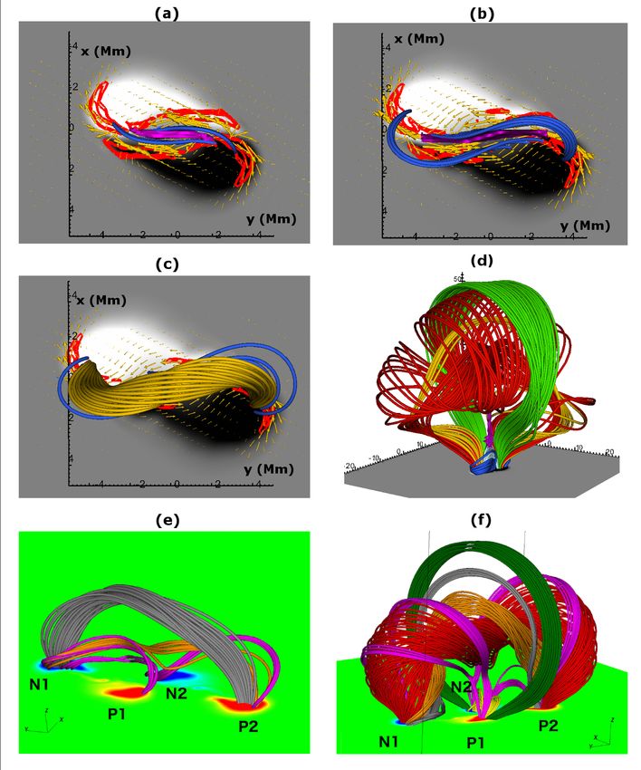
2                                                                S. Patsourakos et al.

the issue conclusively. We demonstrate the approach using MHD simulations and
synthetic coronal images.
    Our key conclusion is that the differentiation of pre-eruptive configurations in
terms of SMAs and MFRs seems artificial. Both observations and modeling can
be made consistent if the pre-eruptive configuration exists in a hybrid state that
is continuously evolving from an SMA to an MFR. Thus, the ’dominant’ nature
of a given configuration will largely depend on its evolutionary stage (SMA-like
early-on, MFR-like near the eruption).
Keywords Plasmas · Sun: activity · Sun: corona · Sun: magnetic fields · Sun:
Coronal Mass Ejections · Sun: Space Weather

1 Introduction

Coronal Mass Ejections (CMEs) are large-scale expulsions of magnetized coronal
plasma into the heliosphere. They represent a key energy release process in the
solar corona, and a major driver of space weather. Despite the observations and
cataloguing of the properties of thousands of events in the last 40 years, the for-
mation and nature of their pre-eruptive magnetic configurations are still eluding
us. Which magnetic configurations are most prone to destabilize and form a CME
and how they arise remain hotly debated questions.
    The pre-eruptive magnetic configuration of CMEs has been modeled either as
a sheared magnetic arcade (SMA) or as a magnetic flux rope (MFR). In some the-
oretical/numerical models, the pre-eruptive configuration is an MFR (e.g., Chen,
1989; Amari et al, 2000; Török and Kliem, 2005) and in some the pre-eruptive
configuration is a SMA (Moore and Roumeliotis, 1992; Antiochos et al, 1999).
    Both of these structures are capable of containing dipped, sheared field lines
above a polarity inversion line (PIL), and so are candidates for the magnetic struc-
ture of a filament channel (defined in Section 1.1). Strong PILs are characterized
by the concentration of most of the shear (i.e., non-potentiality) of the magnetic
field, and hence free magnetic energy therein.
    An important point is that all models predict that the CME will contain an
MFR after eruption. Indeed, MFR-like structures are often detected in CME EUV
(e.g. Dere et al, 1997; Zhang et al, 2012; Vourlidas, 2014) and coronagraphic ob-
servations, (e.g., Vourlidas et al, 2013, 2017) and in in-situ measurements (e.g.,
Burlaga et al, 1981; Nieves-Chinchilla et al, 2018). Since the ejected structure is
an MFR, white-light coronagraphic or in-situ observations should not generally be
expected to provide a direct way to determine whether the pre-eruptive configu-
ration was an SMA or an MFR.
    Although there seem to exist only two possible pre-eruptive magnetic geome-
tries (SMA and MFR), several physical mechanisms (e.g., shearing, flux emergence,
flux cancellation, helicity condensation) can give rise to either of them. There is
a vast literature on the subject but there is no consensus on where and when
given mechanisms may be relevant, if they need to operate alone or in tandem,
and whether they are also the cause or the trigger of the subsequent eruption.
Obtaining a clearer picture of what is the pre-eruptive configuration and how it
forms will have important implications for the physical understanding of CMEs
and the origin and evolution of CME-prolific active regions (ARs). Our improved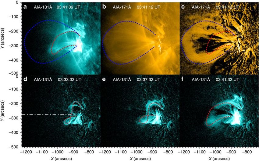
Decoding the Pre-Eruptive Magnetic Field Configurations of CMEs                       3

understanding will help us in turn to better evaluate the eruptivity of a given
AR and hence improve our predictive and forecasting abilities for space weather
purposes (e.g., Vourlidas et al, 2019).
    Despite significant advances in modeling, theory, and observational capabilities,
the resolution of these issues is hampered by a number of factors: (i) limitations
of observations (e.g., lack of routine magnetic-field observations above the photo-
sphere, line-of-sight confusion in imaging), (ii) limitations of models (e.g., idealized
boundary conditions, high numerical diffusion in the MHD codes), (iii) inconsis-
tent application of terms and definitions (defining an MFR in the observations or
the onset time of an eruption, for example) to observations leading to ambiguous
conclusions, and perhaps most importantly (iv), MFRs and SMAs can be nearly
indistinguishable in either field line plots or observations (e.g., filament threads).
    Addressing these issues was the motivation behind the formation of an ISSI
team tasked with ‘decoding the pre-eruptive configuration of CMEs’. The team met
twice with three objectives: (1) debate the formation and configuration of filament
channels, which comprise the observational manifestations of MFRs and SMAs;
(2) identify the open and closed issues; and (3) propose a path forward, for both
modeling and observations, to resolve these issues. The results of our discussions
form the core of this manuscript. We do not attempt to provide a comprehensive
review of CME initiation and formation processes since there exist several recent
excellent reviews on the matter (Chen, 2011; Cheng et al, 2017; Manchester et al,
2017; Green et al, 2018; Archontis and Syntelis, 2019; Georgoulis et al, 2019; Liu,
2020). We focus on three key questions: (1) what constitutes an MFR or SMA?;
(2) how can MFRs/SMAs be identified in the solar atmosphere?; and (3) how do
they form? We compile a set of recommendations for solving these outstanding
issues in the future, whether via modeling or improved observational data.
    This paper is organized as follows. First, we provide definitions for the most
important terms, such as MFR, SMA, Filament Channel, etc., to provide a clear
baseline for the discussion. In Section 2, we review the three dominant mechanisms
for filament channel formation: flux emergence, flux cancellation, and helicity con-
densation. In Section 3, we discuss the modeling expectations and observational
signatures for SMAs and MFRs. In Section 4, we summarize our findings and
provide a table containing MFR/SMA observables that could be checked against
observations. In Section 5, we present recommendations for resolving the nature
of the pre-eruptive configuration and its formation and in the Appendix A we
demonstrate an appropriate methodology using MHD simulations and synthetic
coronal images.

1.1 Basic Definitions

This section contains definitions for the key terms discussed throughout the manuscript.
The definitions are guided by practical considerations, i.e, to help interpret obser-
vations and models.
    Pre-Eruptive Condition: This is the key term for our discussion, yet it is
hard to define precisely. Eruptions occur over a wide range of time scales and
exhibit a variety of signatures at the surface and in the lower atmosphere. For
example, some eruptions precede, others follow, the soft X-ray (SXR) flare onset
4                                                                         S. Patsourakos et al.

Fig. 1 Panel (a): superposed epoch analysis of the velocity-time profiles of 42 CMEs associated
with eruptive flares. The key time of the profiles (i.e., time=0) corresponds to the time of
maximum acceleration for each CME. Modified from Zhu et al (2020) ©AAS. Reproduced
with permission. Panel (b): velocity-time profile of a streamer blowout CME (dashes). Adapted
from Vourlidas et al (2002). In both panels, the horizontal dashed blue lines correspond to a
speed of 100 km/s

and some are not accompanied by flares at all. The timing of, or rather the deter-
mination of whether an eruption is under way, is crucial in assessing the physical
processes responsible for it (ideal or non-ideal, for example). Since there is no
widely-accepted measure or definition of the start of an eruption, we put forth one
as follows. It is logical to expect that a CME will occur when the speed of the
rising structure exceeds a considerable fraction of the local Alfvén speed. At that
point, the rising structure can no longer be considered in a state of a quasi-static
rise caused by, for instance, slow photospheric motions. This quantity is, however,
very difficult to assess observationally or via simulations since the coronal mag-
netic environment is insufficiently known. Instead, we take a more practical, and
conservative, approach and consider a high enough speed to ensure that a CME
will occur across the range of CME source regions. We posit that 100 km s−1 is
a practical limit based on observations of both flare-related and streamer-blowout
CMEs (e.g., Figure 1). Hence, we propose the following definition for the pre-
eruptive condition: The pre-eruption phase ends when the speed of the rising (and
eventually, released) magnetic structure exceeds 100 km s−1 .

Polarity Inversion Line (PIL): The line separating areas of opposite magnetic
polarity on the Sun.
Filament channel (FC): Filament channels are the upper atmospheric coun-
terparts of PILs. They correspond to regions where the magnetic field is largely
aligned with the photospheric PIL. FCs are identified in the chromosphere by
the orientation of chromospheric fibrils. When partially filled with cool and dense
plasma, FCs manifest themselves as filaments or prominences in chromospheric
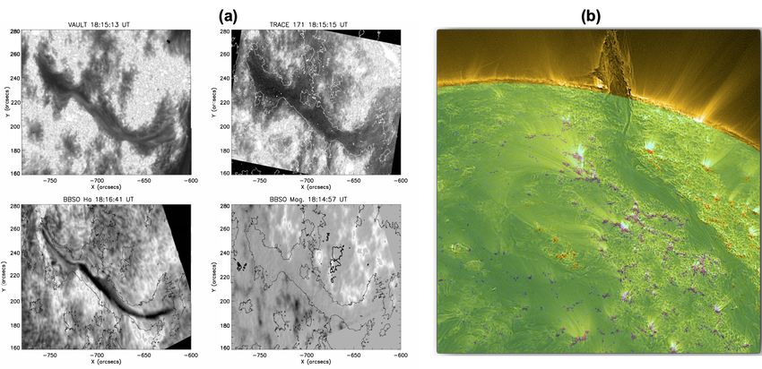
Decoding the Pre-Eruptive Magnetic Field Configurations of CMEs                            5

Fig. 2 Panel (a): A filament channel with prominence material observed in Lyman-α (top
left), 171Å (top right), Hα (bottom left) and photospheric magnetic field (bottom right).
The contours delineate the extent of the Lyman-α prominence. From Vourlidas et al (2010).
©2009, Springer Nature. Panel (b): Composite of AIA 171Å (gold) and HMI magnetogram
(green overlay with positive flux in red and negative flux in blue) of a spectacular filament
channel containing a filament/prominence.

and coronal observations e.g, see Figure 2.

Sheared Magnetic Arcade (SMA): A set of field lines (or flux bundles) that
cross a PIL with an orientation deviating from the local normal to the PIL (see
Section 3.1). An SMA does not have an axis field line about which its flux, or an
inner part of its flux, twists from end to end but it can nevertheless contain a small
amount of twisted flux. In a strongly sheared arcade, the orientation of the field
lines closely follows the PIL. In an SMA, the sheared flux is much larger than the
twisted flux . SMA models range from simple, pseudo-2.5D cases that contain only
arched field lines of the same orientation (Figure 3(a)) to more complex, fully 3D,
cases that contain S-shaped and dipped field lines (Figure 3(b)). In this review,
we mainly discuss these more realistic, complex SMAs.

Magnetic Flux Rope (MFR): A twisted flux tube where the majority of the
interior field lines wind about a common axial field line along the length of the
tube. This is an expanded definition of the textbook MFR (Priest, 2014) to ac-
count for the complexities encountered in current models and their comparisons
with observations, which we discuss in detail in the rest of the paper. MFRs are
characterized by the presence of a magnetic axis, a current channel, and twist ex-
tending over the full length of the magnetic axis (Figure 3(c)). We classify MFRs
based on the twist number N (their end-to-end number of turns) as: 1) weakly
twisted (N < 1); 2) moderately twisted ( N ≈ (1 − 2)); 3) highly twisted (N > 2).
MFRs do not necessarily possess uniform twist, or twist peaking in the vicinity of
the axis (Figure 2(c)) — field lines near the axis can have minimal twist (Figure
2(d)). However the defining MFR characteristic is that the twisted flux is much
larger than the sheared flux . The axis of MFRs relevant to eruptions follows the
PIL relatively closely. For an arched MFR to possess dips, one must additionally
6                                                                          S. Patsourakos et al.

Fig. 3 Pre-eruptive (panels a-e) and eruptive configurations (panels f-g) from MHD simu-
lations. Magnetic fields lines are shown in all panels. Panel (a): 2.5D SMA. Modified from
Zhou et al (2018). Panel (b): 3D SMA. Modified from DeVore and Antiochos (2000). Panel
(c): MFR with twisted field lines concentrated in the core of the configuration. Modified from
Titov et al (2014). Panel (d): MFR with twisted field lines concentrated in the periphery of
the configuration (i.e., hollow-core configuration). Modified from Titov et al (2014). Panel (e):
hybrid configuration. Modified from Török et al (2018a). Panel (f): eruptive MFR from a sim-
ulation employing a pre-eruptive MFR that has evolved from the [hybrid] configuration shown
in panel (e) . Modified from Török et al (2018a). Panel (g): eruptive MFR from a simulation
employing a pre-eruptive SMA. Modified from Lynch et al (2008). All figures are ©AAS and
reproduced with permission.

require at least ∼ 1 end-to-end turn (see Section 3.2 for details). Examples of erup-
tive MFRs resulting from pre-eruptive MFRs or SMAs are given in panels (f) and
(g) of Figure 3 respectively.

SMA-MFR Hybrid: A magnetic configuration that contains both sheared and
twisted flux in non-negligible, and possibly evolving, proportions (Figure 3(e)).
Hybrids can arise in FCs by magnetic reconnection in the center of an SMA (Sec-
tion 2) or between an SMA and its overlying potential loops or by the diversion of
some of the current-carrying flux to localized polarities along the PIL (Section 3.1).

   All three magnetic field configurations above are current-carrying structures
loaded with free magnetic energy and magnetic helicity. Hence, they could all lead,
under specific conditions, to eruptions. In the rest of the paper, we discuss these
conditions, caveats and observational and modelling challenges.
Decoding the Pre-Eruptive Magnetic Field Configurations of CMEs                    7

2 Filament Channel Formation

Filament channels are the cornerstones for understanding solar eruptive activity.
FCs are sheared, and hence are reservoirs of magnetic free energy, which is required
to fuel eruptive phenomena. CMEs occur only above PILs that are traced by an
FC (all CME theories and models require the presence of an FC above a PIL).
Hence, understanding FC formation equates to understanding the pre-eruptive
configuration in the corona. FC properties are reviewed in several papers (e.g.,
Martin, 1998; Mackay, 2015).
    The literature abounds with modeling efforts to explain the formation of the
magnetic configuration of a filament channel (for a comprehensive review, see
Mackay et al, 2010). The models can be differentiated between those employing
surface effects (differential rotation, meridional flows, shear and converging flows,
helicity condensation), and those employing sub-surface effects (the emergence of
MFRs). In particular, FC could be formed by the following three mechanisms:
(a) flux emergence, (b) flux cancellation, and (c) helicity condensation. Note, that
frequently these mechanisms do not operate in isolation. Sections 2.1, 2.2 and 2.3
discuss these mechanisms and the corresponding observations in detail.

2.1 Flux Emergence

2.1.1 Introduction

A number of observational studies have shown that the formation of FCs is related,
implicitly or explicitly, to the process of magnetic flux emergence from the solar
interior into the solar atmosphere. There are studies suggesting that during flux
emergence, a (twisted) flux tube, which rises from the solar interior, can emerge as
a whole above the photosphere (e.g. Lites, 2005; Okamoto et al, 2008; Lites et al,
2010; Xu et al, 2012; Kuckein et al, 2012). This bodily emergence may result in
a pre-eruptive MFR configuration. Other studies have reported that pre-eruptive
structures can form along the strong PILs of ARs during flux emergence. For
instance, the gradual build-up of free energy injected by photospheric motions
can lead to shearing of the emerged magnetic field, forming an SMA. Numerical
simulations of magnetic flux emergence indicate that such an SMA may eventually
evolve into an MFR, which could erupt towards the outer solar atmosphere (e.g.
Manchester et al, 2004; Archontis and Török, 2008; Archontis et al, 2009; Fan,
2009b; Archontis and Hood, 2012; Moreno-Insertis and Galsgaard, 2013; Leake
et al, 2013, 2014; Syntelis et al, 2017, 2019b). Moreover, studies have reported
the formation of FCs at the periphery of ARs or between neighbouring ARs (e.g.
Gaizauskas et al, 1997; Wang and Muglach, 2007).
    Here, we should highlight that the scope of this review is not an extended
presentation of the various aspects of magnetic flux emergence, as a key process
towards understanding the nature of solar magnetic activity. There exist several
comprehensive reviews on this subject (e.g. Moreno-Insertis, 2007; Archontis, 2008;
Fan, 2009a; Nordlund et al, 2009; Archontis, 2012; Hood et al, 2012; Stein, 2012;
Cheung and Isobe, 2014; Toriumi, 2014; Archontis and Syntelis, 2019; Leenaarts,
2020). Thus, in the following sections, we mainly focus on the pre-eruptive struc-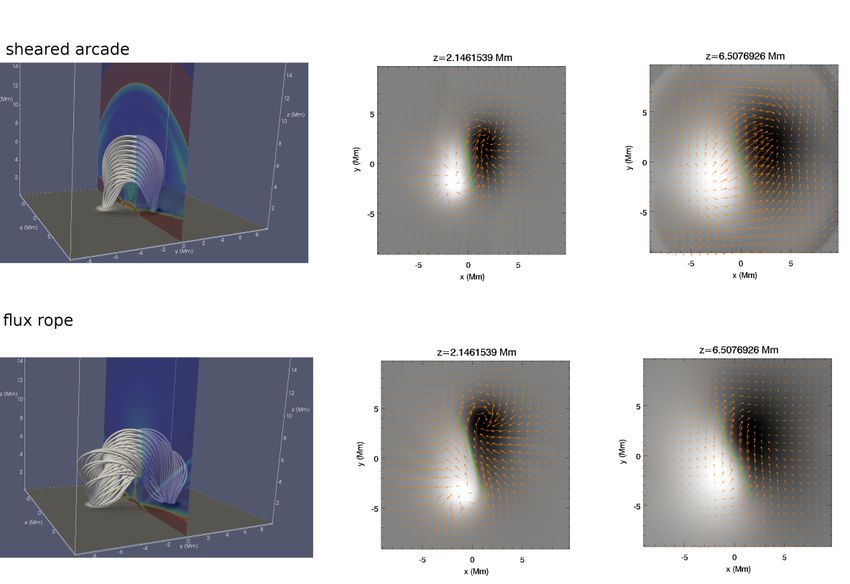
8                                                                 S. Patsourakos et al.

tures that form as a result of flux emergence, from a modelling (section 2.1.2) and
an observational perspective (section 2.1.3).

2.1.2 Flux Emergence Modeling

Numerical experiments of magnetic flux emergence can be classified in two very
broad categories, based on the nature of the background atmosphere that is in-
cluded in the simulations. In the first category, the numerical domain contains the
upper part of the solar atmosphere (e.g., the solar corona), and the magnetic flux
is injected through the lower boundary of the domain, typically in the form of
an MFR (e.g. Fan and Gibson, 2004). Such boundary-driven models are useful to
study the stability and/or the eruptive behavior of coronal structures, but they do
not capture the emergence process itself. In the second category, the magnetic field
emerges from the solar interior and expands into a highly stratified atmosphere
above the photosphere, driving the atmospheric dynamics self-consistently (e.g.
Manchester, 2001; Fan, 2001; Archontis et al, 2004). A typical (idealized) numer-
ical setup for the experiments in the second category consists of a convectively
stable solar interior, a photospheric/chromospheric region of constant tempera-
ture and decreasing density, a region where the temperature increases rapidly
with height, mimicking the temperature gradient of the transition region, and an
isothermal corona. In this review, we will mainly focus on the models of the second
category, as they are more suitable for studying the formation and evolution of
pre-eruptive magnetic structures, at various atmospheric heights.
    The most common initial condition for the sub-photospheric magnetic field is
a twisted flux tube placed in the upper part of the solar interior, adopting the
configuration of a straight horizontal tube or of a torus-shaped tube. Then, the
emergence is initiated by imposing a density deficit along the tube, which makes
part of the tube magnetically buoyant (e.g. Fan, 2001), or by imposing a velocity
perturbation (e.g. Magara and Longcope, 2001, 2003) along a segment of the tube,
which leads to the development of a rising loop with an Ω-like shape (e.g. Archontis
et al, 2004; Manchester et al, 2004). Toroidal flux tubes are typically used to mimic
the top part of a sub-photospheric Ω-shaped emerging loop (e.g. Hood et al, 2009;
Cheung et al, 2010).
    A considerable number of flux-emergence simulations have been using a sub-
photospheric horizontal magnetic flux sheet as initial condition. The interplay be-
tween the effect of convective motions on the magnetic field and the effect of the
distorted field on the motion leads to the development of a series of small-scale in-
terconnected Ω-shaped loops (a ‘sea-serpent’ configuration Pariat et al, 2004)) that
may eventually emerge through the photosphere (e.g. Isobe et al, 2007; Archontis
and Hood, 2009; Toriumi and Yokoyama, 2010; Stein et al, 2011; Stein and Nord-
lund, 2012). These simulations have been used successfully to study small-scale
dynamic phenomena such as Ellerman bombs and UV bursts (e.g., Danilovic et al,
2017; Hansteen et al, 2017, 2019) and the formation of complex bipolar regions and
pores (e.g. Stein and Nordlund, 2012). However, these numerical experiments have
not (yet) been able to produce large-scale pre-eruptive configurations or eruptions.
    We note that a significant number of flux-emergence simulations incorporated
additional physics, such as convective motions, radiative heating and cooling, heat
conduction, ambipolar diffusion, ion-neutral interactions, and non-equilibrium ion-
ization (e.g., Leake and Arber, 2006; Stein and Nordlund, 2006; Cameron et al,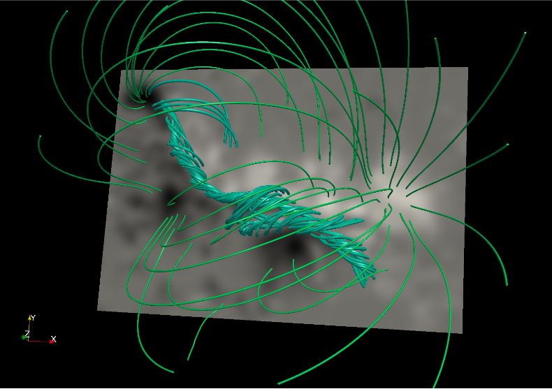
Decoding the Pre-Eruptive Magnetic Field Configurations of CMEs                     9

2007; Martı́nez-Sykora et al, 2008; Isobe et al, 2008; Cheung et al, 2010; Fang et al,
2010; Rempel and Cheung, 2014; Chen et al, 2017; Hansteen et al, 2017; Moreno-
Insertis et al, 2018; Nóbrega-Siverio et al, 2018; Cheung et al, 2019; Toriumi and
Hotta, 2019). These simulations are necessary for studying the thermodynamical
aspects of phenomena related to flux emergence and the atmospheric response
to the dynamic emergence of solar magnetic fields. However, the vast majority
of these experiments have not yet included the solar corona to an extent that is
required to model pre-eruptive configurations.
    In the following, we will review the formation and evolution of the most com-
mon pre-eruptive configurations that are found in flux-emergence simulations.
                   Partial and bodily emergence of MFRs
    Numerical simulations have shown that the rise of an initially horizontal sub-
photospheric flux tube is usually not followed by the bodily emergence of the
tube into the higher atmosphere (e.g., Fan, 2001; Magara and Longcope, 2003;
Manchester et al, 2004). When the top part of a flux tube starts to emerge into
the atmosphere, it expands rapidly due to the pressure difference between itself
and the solar atmosphere. During this expansion, a region with low density and
pressure is formed at the centre of the emerging region, at photospheric heights.
Plasma then drains along the field lines, moving from the top part of the flux tube
towards this low-pressure region (e.g. Manchester et al, 2004) and, eventually, it
accumulates in the dips of the twisted field lines. The dips become heavier and,
thus, the axis of the tube cannot emerge fully into the corona. Rather, it reaches
only a few pressure scale heights above the photosphere. Full (bodily) emergence
can occur only if the tube is buoyant enough to reach the top of the low pressure
region, before the drained plasma accumulates at its dips.
    Magara and Longcope (2003) demonstrated how the curvature of different
field lines within a horizontal flux tube, which emerged from just below the photo-
sphere (-2.1 Mm), affected the draining of plasma. Murray et al (2006) performed
a parametric study in a similar setup, and varied the initial twist (affecting plasma
draining) and the initial magnetic field strength (affecting the buoyancy) of the
sub-photospheric flux tube. More draining and more buoyancy assisted the axis
of the tube to move higher inside the photosphere. MacTaggart and Hood (2009)
studied a case where the middle part of the tube was emerging and the flanks were
submerging. This led to more efficient draining along the flanks of the tube but it
didn’t trigger bodily emergence.
    In all the above-mentioned studies, the initial location of the emerging flux
tube was near the photosphere. Syntelis et al (2019a) imposed horizontal flux
tubes deeper in the solar interior (-18 Mm), to allow the tubes to develop a more
strongly curved shape as they emerge towards the photosphere. They performed
a large parametric study, varying the magnetic field strength, radius, twist, and
length of the buoyant segment of the tube (a proxy for the curvature). They
found that the axis of the flux tube always remained below the photosphere. In
addition, they showed that it is non-trivial to predict the combined effects of these
parameters during the emergence of the field. For instance, a non-intuitive result
was that high-strength (weak-strength) flux tubes may fail (succeed) to emerge
into the atmosphere, depending on their geometrical properties.
    On the other hand, Hood et al (2009) studied the emergence of a weakly
twisted, toroidal flux tube. They found that the geometrical shape of the tube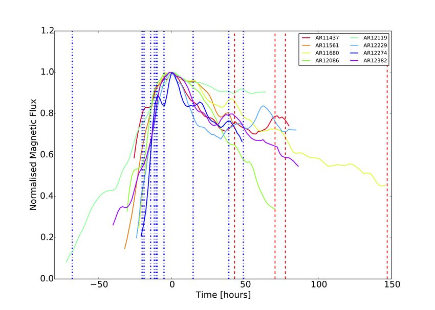
10                                                                   S. Patsourakos et al.

(higher curvature), and the smaller number of dips along the twisted field lines,
triggered sufficient plasma draining and buoyancy, which helped the tube to emerge
bodily into the corona, given that the initial field strength in the tube was chosen
sufficiently strong. MacTaggart and Hood (2009) systematically varied the field
strength and found cases where the axis of the tube (i) could not break through
the photosphere, (ii) emerged but stayed within the photospheric layer, and (iii)
reached coronal heights and continued rising (i.e., emerged bodily). The bodily
emerged MFRs in these simulations appear to be weakly twisted (about one turn
or less), but the dependence of the MFR twist on the initial field strength or twist
of the sub-photospheric flux tube has not yet been studied systematically. Both
Hood et al (2009) and MacTaggart and Hood (2009) reported that a second MFR
formed via magnetic reconnection (see below for a detailed description of this
process) underneath the bodily emerged MFR. If, on the other hand, the original
axis did not emerge into the corona, the second MFR was seen to form above it
(see Figure 4).

Fig. 4 Creation of converging flows during the partial emergence of a sub-surface MFR and
subsequent reorganization of the coronal field, which produces a new MFR. Reproduced with
permission from A&A, ©ESO. From MacTaggart and Hood (2009).

    The numerical experiments summarized in this section suggest that whether a
sub-photospheric twisted flux tube emerges bodily, partially, or not at all, depends
mainly on the properties of the rising magnetic field and its geometric configura-
tion. It appears that bodily emergence requires rather specific conditions, namely
a toroidal geometry and a relatively large field strength. We discuss observational
evidence for bodily emergence in Section 2.1.3. Next, we focus on the formation
of MFRs via magnetic reconnection, as seen in flux-emergence simulations.
                       MFR formation via reconnection
    The emergence of a single sub-photospheric flux tube typically leads to the
formation of a bipolar region, whose polarities separate over time. Photospheric
motions commonly found in the vicinity of the region’s PIL include: (i) shearing
along the PIL, resulting from the Lorentz force developed at the photosphere due
to the expansion of the emerging field (e.g., Fan, 2001; Manchester, 2001), (ii)
rotation of the polarities driven by the propagation of a torsional Alfvén wave
Decoding the Pre-Eruptive Magnetic Field Configurations of CMEs 11 into the atmosphere (e.g., Longcope and Klapper, 1997; Fan, 2009b; Leake et al, 2013; Sturrock et al, 2015; Sturrock and Hood, 2016), and (iii) downflow of plasma towards the low-pressure region above the PIL as discussed above (e.g., Manchester et al, 2004). The combination of these motions induces converging flows towards the PIL (e.g., Archontis and Hood, 2010; Syntelis et al, 2017), which ultimately lead to the formation of an MFR. Fig. 5 MFR formation by reconnection in bipolar and quadropolar regions. (a, b) Top view on field lines that become increasingly sheared and adopt a double-J-like shape (blue lines). The horizontal slice shows the distribution of Bz (black and white) at the photosphere. Over- plotted are yellow arrows showing the photospheric velocity field scaled by magnitude, red contours showing the photospheric vorticity and a purple isosurface showing |J|/|B| = 0.3 (c) Field lines of the sigmoidal MFR formed by reconnected J-like field lines (orange). (d) The field line topology during the eruption of the MFR. The red lines show tether-cut field lines due to reconnection, the green lines show the remaining envelope field which has not yet reconnected and the cyan lines show the post-reconnection arcade. The purple isosurface shows the flare CS. (e) The topology of the field lines in a quadrupolar region. Pink lines show the field lines of the two interacting magnetic lobes. Orange lines have been traced from the close vicinity of the core of the MFR. Field lines in grey color show the ”envelope” field resulting from reconnection between the two magnetic lobes. (f) The field line topology during the rise of the MFR, which is eventually confined by the envelope field. The red lines are field lines, which have been reconnected during the interaction of the two magnetic lobes and the formation and rise of the MFR. The green and grey field lines lines belong to the envelope field above the MFR. The low-lying yellow field lines are reconnected field lines, which form a system of post-reconnection arcade loops that connect the inner polarities (P1, N2).(from Syntelis et al (2017) and Syntelis et al (2019c) ). ©AAS. Reproduced with permission.
12                                                                 S. Patsourakos et al.

    This is illustrated in Figure 5. The described motions inject free magnetic
energy into the system and lead to the gradual formation of an SMA above the PIL.
Eventually, a strong, vertical current layer is formed within the SMA (Figure 5a),
the sheared field lines adopt a double-J shape (Figure 5b), and the current layer’s
strength increases. Field lines that belong to the SMA reconnect above the PIL
and form a (new) MFR with a sigmoidal shape (Figure 5c) at low atmospheric
heights. Spectroscopic observations by CDS,EIS and IRIS, taken at the footprints
of forming MFRs, showed significant line-shifts and line-broadenings, implying the
occurrence of reconnection in the low atmosphere (Foley et al, 2001; Harra et al,
2013; Cheng et al, 2015).
    The newly formed MFRs are typically weakly twisted (approximately one turn,
although the exact number of turns has not been measured in most studies) and
can become eruptive (Figure 5d). Overall, a large number of numerical experiments
(e.g. Manchester et al, 2004; Archontis and Török, 2008; Archontis et al, 2009;
Fan, 2009b; Archontis and Hood, 2012; Leake et al, 2013; Moreno-Insertis and
Galsgaard, 2013; Archontis et al, 2014; Fang et al, 2014; Leake et al, 2014; Lee
et al, 2015; Syntelis et al, 2017; Toriumi and Takasao, 2017; Syntelis et al, 2019b,c)
have shown that post-emergence MFRs can form through reconnection of sheared
magnetic field lines across a current layer above the PIL of an emerging AR, in
the same manner as suggested for the formation of large-scale (quiescent) FCs
suggested by van Ballegooijen and Martens (1989); see also Section 2.2.
    Flux-emergence models have been used to study also the dynamic evolution at
the PILs between colliding/interacting bipoles in quadrupolar ARs (e.g. Fang and
Fan, 2015; Takasao et al, 2015; Toriumi and Takasao, 2017; Cheung et al, 2019;
Syntelis et al, 2019c). We note that the nature of shear and its role for the formation
and eruption of MFRs has been investigated also in observational studies, for cases
of two colliding emerging bipoles (Chintzoglou et al, 2019). Here we focus on the
formation of MFRs in quadrupolar ARs in flux-emergence simulations.
    The most common initial set up of the numerical simulations on this subject
include the emergence of either: (i) a single Ω-loop flux tube with low twist (e.g.
Murray et al, 2006; Archontis et al, 2013; Syntelis et al, 2015); (ii) a single flux
tube emerging at two different locations along its length (“double-Ω” loop), so that
two nearby bipoles appear at the photosphere (e.g. Fang and Fan, 2015; Lee et al,
2015; Toriumi and Takasao, 2017); (iii) two different Ω-loop flux tubes emerging
nearby (e.g. Toriumi et al, 2014; Toriumi and Takasao, 2017); (iv) a single kink
unstable flux tube (such flux tubes, depending on the twist, can form from bipolar
to more complex multipolar configurations) (e.g. Takasao et al, 2015; Toriumi and
Takasao, 2017; Knizhnik et al, 2018). In the above cases, a PIL is formed between
the inner-most polarities of the quadrupole, above which a strong current layer
can build up and a MFR can be formed. Such MFRs can potentially erupt.
    Syntelis et al (2019c) reported on a model of recurrent confined eruptions in a
quadrupolar region. Initially, prior to the formation of the MFR, the two magnetic
lobes above the two emerged bipoles were not interacting. As the bipoles emerged
and moved, the inner polarities of the quadrupole approached each other, and a
current sheet (CS) formed above the PIL between them, extending between the two
magnetic lobes. The strength and size of this CS progressively increased over time.
Reconnection between the two magnetic lobes through that CS formed a magnetic
“envelope” above the quadrupolar region and a weakly-twisted (approximately
one turn) post-emergence low-lying MFR (Figure 5e). This pre-eruptive MFR did
Decoding the Pre-Eruptive Magnetic Field Configurations of CMEs 13
not result from the internal reconnection of a SMA. Rather, the MFR formed
directly. The eruption of the MFR was triggered by reconnection internally within
the quadrupolar region, occurring both below and above the MFR. During the
confined eruption, the weakly twisted low-lying MFR became a larger and more
twisted confined coronal MFR, similar to confined-flare-to-flux-rope observations
(e.g. Patsourakos et al, 2013). The eruptivity of the latter MFR was not studied.
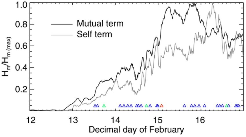
Post-emergence MFRs can form in a recurrent manner as long as the photo-
spheric motions are present and magnetic energy is injected into the system (e.g.
Moreno-Insertis and Galsgaard, 2013; Archontis et al, 2014; Syntelis et al, 2017,
2019b,c). When the driving motions are no longer able to build enough free en-
ergy, the recurrent formation of post-emergence MFRs ceases. It is important to
note here that in flux-emergence models, the formation of MFRs and subsequent
eruptions do not occur only during the flux-emergence phase (i.e., while the pho-
tospheric flux still increases). They can also occur when the photospheric flux has
saturated, but the photospheric motions are still present (e.g, the vertical dashed
lines in Figure 20 in the Appendix).
As we have mentioned previously in this section, the pre-eruptive MFRs are
typically weakly twisted. However, we should highlight that the number of turns of
the field lines resulting from the reconnection between two flux systems depends on
the specifics of the reconnection region. For instance, Wright (2019) showed that:
a) the relative orientation of the footpoints of the two pre-reconnection flux sys-
tems and b) their magnetic helicity content (for a discussion on magnetic helicity
see Section 2.3), are crucial to determine the resulting twist after they reconnect to
each other. These two factors affect how self-helicity is partitioned between the re-
sulting post-reconnection systems. Wright (2019) discussed cases where the twist of
the resulting two flux systems can increase, decrease or remain the same after their
interaction. Priest and Longcope (2020) further studied how self-helicity is parti-
tioned between reconnecting systems, by examining twist during the reconnection
of flux sheets, sheaths and tubes, and discussed how the twist of the erupting MFR
increases during the eruption, leaving behind an untwisted arcade. Multiple recon-
nection events between different flux systems can furthermore increase/decrease
the twist of a pre-eruptive MFR. This can occur when the post-reconnected field
lines reconnect again with field from the same pre-reconnected systems, or when
they reconnect with other flux systems. Similarly, during an eruption, the MFR
twist typically increases due to multiple reconnection events in the flare CS be-
low the core of the erupting MFR (e.g., red lines in Fig. 5d and Gibson and Fan
(2006b); Syntelis et al (2017); Inoue et al (2018); Syntelis et al (2019b)).
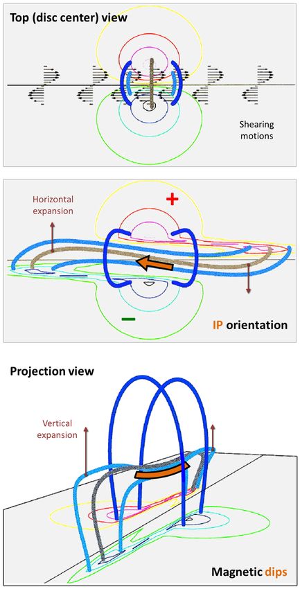
MFRs could also form at the periphery (or in between) ARs as was recently
suggested by Török et al (2018b). They modeled the emergence of an MFR close
to a pre-existing bipolar AR. The orientation of the MFR was chosen such that a
quadrupolar configuration with a current layer between the pre-existing and newly
emerged flux systems resulted, similar to the configurations just described. A pair
of so-called “conjoined flux ropes” (CFRs; e.g., Wyper and Pontin, 2014b,a; Titov
et al, 2017; Fu et al, 2017) was created by the tearing instability in the current
layer and advected to the lower atmosphere, leading to the formation of two MFRs
of opposite axial-field direction (i.e., opposite helicity sign) that are located end-
to-end above the “external” PIL section between the new and pre-existing flux
(Figure 6). Note that the CFRs form in addition to the main MFR that bodily
emerges or forms above the “internal” PIL of the emerging region, as described14 S. Patsourakos et al.
Fig. 6 MHD simulation of FC formation at the periphery of an emerging AR. (a) Top view
on the AR, which emerges into a positive background field, close to a pre-existing AR (not
shown). The yellow line marks the PIL, arrows show the horizontal magnetic field (magenta)
and current density (green) along the external PIL section. The magnetic field switches sign
along and above this section (indicated by black arrows), leading to the formation of CFRs
(i.e., two adjacent MFRs of opposite helicity sign) via reconnection across the current layer
(indicated in cyan). (b) Oblique view on the MFRs, colored by α = (j · B)/B 2 . The location
of the spiral null point between the two MFRs is illustrated by a thick field line.
above. Note also that the presence of a pre-existing bipole is not required for
this mechanism to work, as the current layer forms between the inner polarities.
That is, the mechanism can work also when an AR emerges within, or close to, a
single-polarity region, i.e., a coronal hole.
2.1.3 Flux emergence observations
We start with observations of FC formation within the cores of emerging flux
regions interpreted in favor of bodily emerging MFRs. Lites et al (1995) studied the
emergence and evolution of a small δ-spot AR, where a low-lying filament was seen
in Hα above the PIL. They found that a “magnetically closed structure” remained
in the corona even after the disappearance of the δ-spot AR. They attributed this
to an MFR in equilibrium with the ambient coronal field, after it had emerged
through the photosphere. Later works revisited the emerging MFR scenario by
examining the vector magnetic field in locations where filaments form in plages,
at the photosphere (Lites, 2005; Okamoto et al, 2008; Lites et al, 2010) and by
also including chromospheric vector magnetograms (Kuckein et al, 2012; Xu et al,
2012). The photospheric vector field in these works is found to be of a “concave-
up” geometry suggesting a magnetic structure dipping at the PIL, and also that
of an “inverse” horizontal field (with respect to that of a potential field, which
is called “normal”) crossing the PIL. To our knowledge, these works are the only
references suggesting full (i.e., bodily) MFR emergence, making it a rather scarce
observation.
However, several important observational limitations (e.g., incomplete spectral
and temporal coverage or confusion from pre-existing structures and the lack of
multi-height vector magnetic field measurements), do not allow to unambiguously
interpret observations of flux emergence. Therefore, their interpretation in terms
of bodily emerging MFRs could not be unique.Decoding the Pre-Eruptive Magnetic Field Configurations of CMEs 15
For example, several analyses take place while a filament already exists in
these locations (Okamoto et al, 2008; Kuckein et al, 2012), casting doubt that
these are studies of true FC formation. In addition, MHD modeling of dynamic
emergence of a twisted cylinder into an overlying arcade by Vargas Domı́nguez
et al (2012) showed the same photospheric signatures as observed by Okamoto
et al (2008). However, this was not a case of a bodily-emerging flux rope into
the corona, since the axis of the emerging cylinder reached only one photospheric
scale-height above the photosphere. This result reveals that the concave upward
geometry is not an exclusive indication of a bodily emerging MFR. The Xu et al
(2012) study was based on the analysis of a single chromospheric magnetogram (in
HeI 10830 Å) and comparison to Hα. They found that the chromospheric magnetic
field exhibited the normal configuration while the photospheric magnetic field was
concave upwards and these results were interpreted in terms of bodily emergence
of a flux rope that is producing a filament. The authors acknowledge that their
interpretation is not unambiguous given that the observed differences in HeI 10830
Å and Hα may be interpreted in terms of optical-depth effects. The same issue
affects the Kuckein et al (2012) results since they used the same lines. Mackay
et al (2010) analyzed the same sequence as Okamoto et al (2008) but interpret the
signatures in the Ca II H line being due to a rising SMA rather than an MFR.
Lites et al (2010) discuss the possibility of surface flows creating their observed
short-lived filament channel via cancellation, but they reject it based on the lack of
systematic photospheric flows that could produce significant shear and convergence
along the channel. However, their flow field was determined from the photospheric
granulation instead of tracking magnetic elements in magnetograms. Therefore,
MFR formation by flux cancellation (see next section) remains a candidate.
We now pass into a discussion of observations of FC formation in the periphery
of ARs, rather in their cores, including quiet Sun (QS) filaments. AR periphery is
indeed where most filament channels form. Observations, (e.g., Gaizauskas et al,
1997; Wang and Muglach, 2007), suggest that such filament channels form during
mainly interactions of emerging bipoles with existing ones. The bipoles converge
and flux cancellation and reconnection take place. These scant observations, along
with the considerations of the solar-cycle characteristics of filament channels within
and outside ARs, with only the latter showing solar-cycle dependence, led Mackay
et al (2010) to conclude that emerging flux ropes are not relevant for the forma-
tion of filament channels outside ARs, and ”surface” phenomena, i.e., converge
and cancellation are more pertinent. We finally note here, that the observational
inferences of bodily emerging flux ropes within AR cores discussed in the previous
paragraphs, may not be attainable for the case of filament formation outside ARs,
given the weaker (horizontal) magnetic fields in these areas.
Flux emergence in multipolar ARs can eventually lead to the formation of
MFRs (Chintzoglou et al, 2019). These authors reported observations of multiple
bipoles, emerging either simultaneously or sequentially, in two emerging ARs. The
collision between oppositely signed nonconjugated polarities (i.e., polarities not
belonging to the same bipole) of the different emerging bipoles within the same
AR gave rise to shear and flux cancellation, hence this process was called collisional
shearing. Photospheric flux cancellation and reconnection above the photosphere
in the PIL(s) undergoing collisional shearing progressively converted SMAs into
pre-eruptive MFRs and produced intense flare clusters for the duration of colli-
sion. In the same study, a data-driven evolutionary magneto-frictional model (e.g.,16 S. Patsourakos et al.
Fisher et al, 2015) was applied to time-series of photospheric vector magnetic field
and Doppler measurements of the two analyzed ARs, and it was able to capture
and reproduce the various stages of collisional shearing, including the progressive
conversion of SMAs to pre-eruptive MFRs. In addition, using Doppler observations
it was determined that the active part of the AR PIL showed downflows, further
supporting that the pre-eruptive MFRs did not emerge bodily and were produced
by strong cancellation.
2.1.4 Outstanding Issues
We conclude this section with a list of pending issues with regards to flux emer-
gence simulations and observations:
- improve the physical realism of flux emergence simulations;
- lack of systematic studies of full and partial flux-tube emergence ;
- lack of systematic calculations of twist in flux emergence simulations;
- properties and eruptivity of bodily emerging MFRs has not been studied yet;
- lack of extensive surveys looking for bodily emerging MFRs ;
- lack of extensive surveys of FC formation at AR peripheries.
A detailed roadmap towards addressing these issues is given in Section 5.
2.2 Flux Cancellation
2.2.1 Introduction
Magnetic flux cancellation, whereby small-scale opposite magnetic polarities con-
verge, collide and then subsequently disappear (Martin et al, 1985) is a process
ubiquitous all over the solar photosphere (Livi et al, 1985). Flux cancellation takes
place along the PIL (Babcock and Babcock, 1955) that separates negative and
positive photospheric polarities. In particular, cancellation can occur along the in-
ternal PIL of an AR, at an external PIL formed at the AR periphery, or in the QS.
According to the classical picture of magnetic flux cancellation described in van
Ballegooijen and Martens (1989) it invariably leads to the formation of an MFR.
A different model for magnetic cancellation is discussed in Section 2.3, and when
combined with helicity condensation, this type of cancellation leads to an SMA.
2.2.2 Flux cancellation modeling
Flux cancellation due to magnetic reconnection at the surface is typically mod-
eled by modifying the lower boundary of a simulation domain that represents
the photosphere. For example, in the work of Amari et al (1999); Linker et al
(2001); Lionello et al (2001), a potential-field extrapolation of either an idealized
or observed AR magnetic field is used as the initial condition. This field is then
energized by surface flows, such as shearing or twisting, followed by diffusion of the
normal magnetic field on the surface, which is achieved by imposing an appropri-
ate tangential electric field. The ensuing evolution produces a coronal MFR with
dipped field lines that could support filament material. In the model of DeVore
and Antiochos (2000), no specific surface flux cancellation is specified. Instead,
the expansion due to footpoint motions which increase the pressure of the shearedDecoding the Pre-Eruptive Magnetic Field Configurations of CMEs 17
magnetic field in the corona leads to magnetic reconnection, similar to the theo-
retical mechanism of van Ballegooijen and Martens (1989). Finally, in the models
of Yeates et al (2008) and van Ballegooijen et al (2000), diffusion of the magnetic
field at the coronal base (with the simultaneous absence of magnetic diffusion in
the corona) concentrates magnetic field just above PILs, which becomes the axial
field of the MFR formed by the subsequent reconnection.
The complex physical mechanisms associated with flux emergence are reviewed
in Section 2.1. During the partial emergence of magnetic flux (where mass-laden
portions of magnetic flux tubes remain rooted at the surface), the Lorentz force
associated with expanding field lines that are able to drain material produces shear
flows at and above the PIL (Manchester et al, 2004). In addition, because of the
rapid horizontal expansion of the magnetic field at the β = 1 surface (see Figure
4), convergent flows can also be created by the self-consistent evolution of the
magnetic field in the low atmosphere, leading to magnetic reconnection at those
locations (MacTaggart and Hood, 2009). Furthermore, the emergence of concave-
up field lines (U-loops) can occur when the magnetic field becomes significantly
distorted during its emergence in the turbulent convection zone (Magara, 2011).
Therefore, flux emergence can create the observational signatures of shearing and
converging flows, and of flux cancellation.
Recently, the ability to include into the simulations the physical mechanisms
of both flux emergence and flux cancellation due to both magnetic-field evolution
and magneto-convection has been developed. By mimicking the radiative losses at
the surface and including a thermal injection of energy at the base of the simula-
tion domain, MHD simulations spanning a shallow convection zone to lower corona
can now include reasonably realistic convective motions. Fang et al (2012) address
the emergence of MFRs modified by the turbulent convection zone. Within the
emerging structure, converging motions at the PIL, driven by a combination of
magnetic-field evolution and granular motion, cause flux cancellation at the pho-
tosphere, which, along with tether-cutting reconnection in the corona, continues
to build up sheared field lines in the corona. This type of study, performed on real-
istic solar AR timescales may help to understand what causes the flux cancellation
observed prior to internal filament eruptions.
Convective motions at the surface may also aid in the formation of filament
channels both within and external to an AR, via the recent theoretical model of
helicity condensation, discussed in Section 2.3.
2.2.3 Flux cancellation observations
The convergence of opposite magnetic polarities towards PILs that leads to flux
cancellation is driven by the dispersion of decaying AR magnetic fields, through
convection and emergence of AR bipoles into pre-existing magnetic field, and also
by the collision of bipoles during the emergence of multipolar ARs. The process of
flux cancellation is often observed leading up to the formation of filament chan-
nels, filaments and CMEs (Martin et al, 1985, 2012; Martin, 1998; Gaizauskas
et al, 2001; Gaizauskas, 2002; Wang and Muglach, 2007; Mackay et al, 2008, 2014;
Chintzoglou et al, 2019), suggesting that flux cancellation plays an important
role in the construction of pre-eruptive magnetic-field configurations. Small-scale
brightenings and jets have been observed in the corona in connection with can-
cellation sites (e.g., Wang and Muglach, 2013). However, such brightenings are18 S. Patsourakos et al.
most commonly observed in Hα and He II, with fainter or no signatures in coronal
emissions.
There are currently three proposed scenarios that describe the physical pro-
cesses that lead to flux cancellation (Zwaan, 1987): U-loop emergence (van Driel-
Gesztelyi et al, 2000; Bernasconi et al, 2002), Ω-loop submergence (Harvey et al,
1999; Chae et al, 2004; Yang et al, 2009; Takizawa et al, 2012), and magnetic
reconnection taking place low in the solar atmosphere followed by Ω-loop submer-
gence (van Ballegooijen and Martens, 1989). Current observations cannot easily
distinguish between these possibilities.
In the case that flux cancellation is associated with magnetic reconnection, as
in the van Ballegooijen and Martens (1989) model, then sheared magnetic fields
reconnect in the PIL leading to the formation of twisted field lines pertinent to
a MFR. More specifically, the sheared field evolves from an SMA to two sets of
loops that form a “double-J” shape with a low-emission channel between them.
The low emission channel is expected to contain cooler plasma (about 1MK), but
this has not yet been detected. From this configuration, the inner end points of the
two J’s merge and a continuous S-shape forms, but this may also be a projection
effect. This continuous S-shape corresponds to a SXR or extreme ultraviolet (EUV)
sigmoid. Green and Kliem (2014) show this evolutionary scenario for four ARs,
with the transition from SMA to double-J to continuous S-shape typically taking
a couple of days. The continuous S structure is highly supportive of the presence
of an MFR with helical field lines with around one turn, where heated plasma is
confined. However, the MFR may also be present at the time of the two J’s. The
double-Js then represent remnant SMA field that is wrapping around the forming
MFR but which has not yet undergone reconnection and been built into the MFR.
During flux cancellation an amount of flux equal to the amount removed from
the photosphere is available to be built into an MFR. Therefore, flux cancellation
observations present a way to investigate how much magnetic flux has been built
into an MFR before its eruption and we hereby discuss such estimates. Previous
observational studies of flux cancellation monitoring the magnetic flux evolution
in the photosphere, suggest that around 30-50% of the AR flux cancels on average
2-4 days prior to the occurrence of a CME (Green et al, 2011; Baker et al, 2012;
Yardley et al, 2016, 2018a). However, these values represent an upper limit as
the amount of flux that is built into an MFR is dependent on the AR properties,
such as the shear of the magnetic field and the length of the PIL along which flux
cancellation is taking place (Green et al, 2011).
In addition, static or time-dependent (non-linear force-free field; NLFFF) mod-
els provide an alternative method to probe how much flux is contained in an MFR
before its eruption. The models include the flux rope insertion method (van Bal-
legooijen, 2004) to produce a NLFFF extrapolation or the NLFFF evolutionary
model of Mackay et al (2011), to model pre-eruptive configuration of the magnetic
field. Using these models it is possible to investigate the ratio of axial and poloidal
(i.e., at planes perpendicular to the axis ) flux in the MFR to that of the overlying
field for stable and unstable MFRs. Previously, the limit for the axial flux in an
MFR that can be held in stable force-free equilibrium by the overlying field of the
AR was found to be up to 10-14% (Bobra et al, 2008; Su et al, 2009; Savcheva
and van Ballegooijen, 2009). On the other hand, more recent studies that combine
both observations and models have suggested that 20-50% of the AR flux could be
contained in a stable MFR (Savcheva et al, 2012; Gibb et al, 2014). There may beDecoding the Pre-Eruptive Magnetic Field Configurations of CMEs 19
also poloidal magnetic flux added to the MFR via reconnection in the transition
region or corona, but lack of routine magnetic field observations at these layers
prevents any direct assessment of it.
For sigmoids that form along the internal PIL of decaying ARs, the coronal field
appears to follow a systematic evolution when viewed in SXR observations. These
regions match closely the mechanism of van Ballegooijen and Martens (1989) in
that they exhibit flux cancellation along the PIL and an increasingly sheared field
in the corona. A recent study by (Savcheva et al, 2014) has shown that the eruptive
activity of 72 sigmoidal ARs is more strongly correlated with flux cancellation than
with emergence. The study found that 57% of the sigmoids were associated with
flux cancellation compared with only 35% occurring as a result of flux emergence.
The rest of the regions showed a fairly constant magnetic flux evolution.
A secondary effect of flux cancellation is that it reduces the magnetic flux that
contributes to the overlying, stabilizing field of the MFR. If enough flux is can-
celled from the overlying field and incorporated into an MFR, a force imbalance
occurs, which leads to a catastrophic loss of equilibrium and a CME (e.g., Lin
and Forbes, 2000; Bobra et al, 2008). Or, if the overlying field of the AR decays
rapidly enough with height, the flux rope can become torus-unstable (Kliem and
Török, 2006; Török and Kliem, 2007; Démoulin and Aulanier, 2010; Kliem et al,
2014a). Previous observational studies of flux cancellation have found a ratio of
flux contained in the MFR compared to the overlying arcade of 1:1.5 (Green et al,
2011) and 1:0.9 (Yardley et al, 2016). Yardley et al (2018a) recently conducted a
comprehensive study of the CME productivity in a sample of 20 bipolar ARs in
order to probe the role of flux cancellation as a CME trigger. The magnetic flux
evolution was analyzed during the full AR evolution spanning from emergence to
decay. This study found that the ratio of flux cancelled available to be built into an
MFR before eruption compared to the remaining, overlying field was found in the
range 1:0.03 to 1:1.57 for ARs that produced low-altitude CMEs originating from
the internal PIL. The small ratios imply that the assumption that the amount of
flux cancelled is equal to the amount of flux injected into the flux rope does not
necessarily apply here. This needs further investigation. They suggest that a com-
bination of the convergence of the polarities, magnetic shear and flux cancellation
are required to build a pre-eruptive configuration and that a successful eruption
depends upon the removal of a sufficient amount of the overlying field that sta-
bilizes the configuration. The study also showed that the type of CME produced
depends upon the evolutionary stage of the AR. CMEs originating above external
PILs (between the periphery of the AR and the QS) occurred during the emer-
gence phase of the AR, whereas, CMEs originating above an internal PIL of an
AR occurred during the region’s decay phase (see Figure 7).
Note that the majority of the observational studies of flux cancellation dis-
cussed above refer to bipolar and decaying ARs. Flux cancellation can also occur
in multipolar and emerging ARs (Chintzoglou et al (2019) and discussion of Sec-
tion 2.1.3). We note that measuring flux cancellation in periods of flux emergence
is challenging (in comparison to measuring cancellation in decaying ARs) because
the magnetic flux is increasing during the emergence phase. By tracking oppo-
site polarity footpoints and the flux balance of multiple emerging bipoles within
the same AR undergoing collisional shearing (see Section 2.1.3) it was found by
Chintzoglou et al (2019) that amounts of magnetic flux of up to ≈ 40 % of the
net magnetic flux of the smaller emerging bipole may be cancelled. The reportedYou can also read