Single-shot Stern-Gerlach magnetic gradiometer with an expanding cloud of cold cesium atoms
←
→
Page content transcription
If your browser does not render page correctly, please read the page content below
Single-shot Stern-Gerlach magnetic gradiometer with an expanding cloud of cold cesium atoms
Katja Gosar,1, 2 Tina Arh,1, 2 Tadej Mežnaršič,1, 2 Ivan Kvasič,1 Dušan Ponikvar,1, 2 Tomaž
Apih,1 Rainer Kaltenbaek,2 Rok Žitko,1, 2 Erik Zupanič,1 Samo Beguš,3 and Peter Jeglič1, ∗
1
Jožef Stefan Institute, Jamova 39, SI-1000 Ljubljana, Slovenia
2
Faculty of Mathematics and Physics, University of Ljubljana, Jadranska 19, SI-1000 Ljubljana, Slovenia
3
Faculty of Electrical Engineering, University of Ljubljana, Tržaška cesta 25, SI-1000 Ljubljana, Slovenia
(Dated: February 23, 2021)
We combine the Ramsey interferometry protocol, the Stern-Gerlach detection scheme, and the use of elon-
gated geometry of a cloud of fully polarized cold cesium atoms to measure the selected component of the
magnetic field gradient along the atomic cloud in a single shot. In contrast to the standard method where the
arXiv:2011.09779v2 [physics.atom-ph] 19 Feb 2021
precession of two spatially separated atomic clouds is simultaneously measured to extract their phase difference,
which is proportional to the magnetic field gradient, we here demonstrate a gradiometer using a single image of
an expanding atomic cloud with the phase difference imprinted along the cloud. Using resonant radio-frequency
pulses and Stern-Gerlach imaging, we first demonstrate nutation and Larmor precession of atomic magnetiza-
tion in an applied magnetic field. Next, we let the cold atom cloud expand in one dimension and apply the
protocol for measuring the magnetic field gradient. The resolution of our single-shot gradiometer is not limited
by thermal motion of atoms and has an estimated absolute accuracy below ±0.2 mG/cm (±20 nT/cm).
PACS numbers: 03.75.Mn, 05.30.Jp, 07.55.Ge, 67.85.-d
I. INTRODUCTION clouds of cold atoms was demonstrated in Ref. 19. The exper-
imental setup allowed the control of cloud positions, thereby
Atomic magnetometers are among the most precise devices enabling the measurement of the complete magnetic field gra-
for measuring magnetic fields [1, 2]. The magnetic field mag- dient tensor. In inhomogeneous magnetic field the precession
nitude is determined by the Larmor precession frequency of frequency is position dependent. For uniform initial phase,
spins that is proportional to the field they are subjected to. the phase difference between the clouds at positions r~1 and r~2
Centimeter-sized alkali-vapor magnetometers can be applied accumulates with time as:
to measure the magnetic field either as a vector quantity or as ∆φ(t) = γ B(~ r1 ) t ≈ γt (~
r2 ) − B(~
r2 − r~1 ) · ∇B. (1)
a scalar magnitude, depending on the method. They can reach
magnetic field sensitivity as high as 160 aT/Hz1/2 [3]. Here, γ denotes the gyromagnetic ratio. The phase differ-
Ultracold atoms are very suitable for high-precision mea- ence is therefore proportional to the spatial derivative of the
surements due to their long lifetimes and small Doppler broad- magnetic field strength B along the direction connecting both
ening [4]. The sensitivity of cold-atom magnetometers does probes. Traditionally, a series of measurements with incre-
not reach that of the best alkali-vapor devices because of the menting interrogation (precession) times is required to deter-
small size of atom clouds at comparable densities, but they are mine the time evolution of the phase difference. Special care
suitable for measurements with a high spatial resolution. They has to be taken to properly count the integer multiples of 2π
can reach 8.3 pT/Hz1/2 magnetic field sensitivity on a ∼ 10 µm [19].
scale [5], and they can detect magnetic-field inhomogeneities Here we demonstrate a method for measuring the selected
down to 200 nT/cm [6]. Typically, cold-atom magnetometers component of the magnetic field gradient with a single shot,
are based on the same signal detection technique as room- using only one elongated atom cloud instead of two spatially
temperature atomic-vapor magnetometers, i.e., the Faraday separated clouds. Specifically, we measure the spatial profile
rotation [7–14]. This is, however, not the only possibility of the magnetic field through the spatial dependence of the
for detecting the spin precession in cold-atom clouds. Vari- phase difference ∆φ(x, t) along the cloud elongated in the x-
ous techniques have been developed, including state-selective direction, see Fig. 1(a). For a given precession time t, the mag-
phase-contrast imaging [5, 15] and state-selective absorption netic field gradient causes the accumulated precession phase
imaging [6]. Finally, the projection of the magnetization can to have a continuous variation along the atom cloud. We
also be measured through the populations of Zeeman sub- choose the magnetic field B0 to be oriented in the x-direction.
levels using the Stern-Gerlach method, in combination with In this case, we can approximate the position dependence of
using the Ramsey sequence to control the precession time the magnetic field magnitude with B(x) ≈ B0 + (∂Bx /∂x)x.
[16–19]. This is the approach adopted in this work. Here, we neglect contributions from magnetic field gradients
A basic gradiometer consists of two magnetometer probes ∂By /∂x and ∂Bz /∂x, which may result in small magnetic-field
separated in space, and the magnetic gradient is obtained by components perpendicular to the dominant B0 . The magneti-
differentiating their outputs. Magnetic gradiometry using two zation of the atoms in the cloud undergoes a Larmor preces-
sion in the magnetic field. Therefore, its y-projection can be
written as
∂Bx
!
∗ peter.jeglic@ijs.si My (x, t) = M0 cos γB0 t + γ xt . (2)
∂x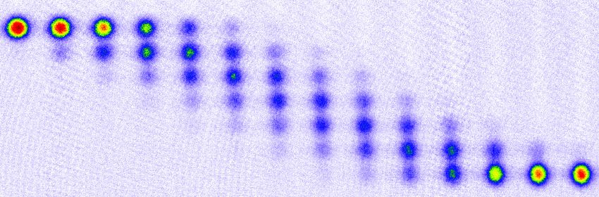
2

Here we assume that, at t = 0, the whole cloud is fully polar-
ized along the y-direction with initial magnetization M0 . As
we show below, a single experimental run with only one Stern-
Gerlach image of the atom cloud is sufficient to obtain My (x)
at the selected precession time t, allowing an unambiguous ex-
traction of the magnetic field gradient ∂Bx /∂x. If the magnetic
field B0 is oriented in other directions, additional components
of magnetic-field-gradient tensor can be determined. For ex-
ample, to determine ∂By /∂x, the magnetic field B0 has to be
in the y-direction.
   According to Eq. (2), nonzero components of the magnetic
field gradient along the cloud cause a helical or ”corkscrew”
spatial dependence of the magnetization direction that can
also be observed in Bose-Einstein condensates [15, 16]. It
is important to note that the time-fluctuations of the mag-
netic field B0 and any non-compensated homogeneous exter-
nal fields contribute only to the overall phase in My (x, t). In
elongated condensates, the phase difference can also become
spatially dependent in the presence of inhomogeneous inter-
nal magnetic fields caused by the spatially modulated struc-
ture of spin domains [20–23], presumably induced by long-
range dipole interaction. In contrast, recent non-destructive
Faraday-rotation experiments showed no spontaneous domain
formation in a tightly confined low-density 87 Rb condensate
[24]. In cold atom clouds, which have even lower densities,
these effects can be neglected.
   In this work, we focus on the detection of magnetic field
gradients originating from external sources. A related tech-
nique is described in Ref. 6, where an elongated but non-
expanding cloud of 87 Rb cold atoms is polarized with a pump        FIG. 1. (a) Schematic illustration of the magnetic gradiome-
beam pulse and the projection of the magnetization is detected      ter showing an elongated 133 Cs cold atom cloud expanded along
with state-selective imaging. In our 133 Cs experiment, the         the dimple beam. (b) The experimental sequence for observing
                                                                    position-dependent Larmor precession of magnetization, caused by
magnetization of the expanding cloud is already fully polar-
                                                                    the ∂Bx /∂x component of the magnetic field gradient. First, the mag-
ized along the applied magnetic field, and we start the pre-        netic field is switched from the z- to the x-direction, then the atom
cession with a pulse of a radio-frequency (RF) magnetic field.      cloud is released to expand along the beam. Next, we use the Ram-
To measure My (x, t) we perform the Stern-Gerlach imaging           sey sequence composed of two π/2 RF pulses that are separated by
(Fig. 1), where we apply a magnetic field gradient to sep-          the interrogation time T R . Finally, the absorption image is taken after
arate the atoms in different Zeeman sublevels and calculate         the Stern-Gerlach separation of mF -state populations in the applied
the magnetization from the atom populations in each sublevel.       magnetic field gradient ∂Bz /∂z.
After taking into account the effect of the cloud expansion dur-
ing the protocol for measuring the magnetic field gradient, we
reach an absolute accuracy below ±0.2 mG/cm (±20 nT/cm)             fully polarized along the x-direction. We prepare cold 133 Cs
in a single shot. The sensitivity of magnetic field gradient is     atoms by laser cooling with a standard procedure described
enhanced by an order of magnitude compared to Ref. 6, where         in detail in Ref. 25, including the transfer of fully polarized
they had ∼ 5 times more atoms in ∼ 10 times more elongated          atoms in the (F = 3, mF = 3) state from a large dipole trap to a
cloud, albeit at ∼ 20 times higher temperatures, which only         small dimple trap with trap frequencies 2π×(20, 120, 120) Hz,
allowed much shorter interrogation times (below 1 ms). As           followed by further evaporative cooling for 100 ms. The re-
discussed below, the resolution of our gradiometer is not lim-      sulting cloud in the dimple trap typically consists of 2 × 10⁵
ited by thermal motion (diffusion) of atoms since their in-trap     cesium atoms at T = 1.29 ± 0.02 µK, with the 1/e radii of
velocity distribution is mapped into well-defined atom trajec-      σ x0 = 69 ± 2 µm and σy0 ∼ σz0 = 12 ± 2 µm. To create
tories during the cloud expansion.                                  an elongated atom cloud one of the dimple beams is turned
                                                                    off and the cloud starts expanding in the x-direction, along the
                                                                    remaining beam (Fig. 1). As shown below, a regime of linear-
                      II.   EXPERIMENT                              in-time expansion is reached after ∼ 20 ms of time-of-flight
                                                                    (TOF). At 40 ms of total expansion time, the cloud extends
  Most cold atom magnetometers and gradiometers are based           over an 1/e length of σ x = 366 ± 3 µm.
on 87 Rb atoms in F = 1 or F = 2 hyperfine states. Here, we            Immediately after the evaporation, we turn off the
use 133 Cs atoms in their F = 3 ground state; initially, they are   quadrupole coil producing a strong magnetic field gradient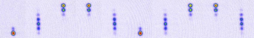
3
of ∂Bz /∂z = 31.3 G/cm used to levitate the cesium atoms component of the spin and its variance will be functions of x:
(Fig. 1(b)). We also turn off the Helmholtz coil produc- hS z (x)i and h∆2 S z (x)i.
ing a homogeneous magnetic field Bz = 22 G, which opti-
mises the cesium scattering length during the evaporation. At
the same time we turn on the compensation coils that can-
cel out the components of magnetic field in the y- and z- III. RESULTS
directions and set the magnetic field in x-direction to a value
of B0 = 143 mG. That corresponds to a Larmor frequency of
ω0 = γB0 = 2π × 50 kHz (γ = 350 kHz/G). Since the induc- Fig. 2(a) shows the oscillations of the mF -state populations
tances of the quadrupole, Helmholtz and compensation coils of 133 Cs atoms in the F = 3 hyperfine state measured by
are large (the switching times are in the order of several ms), the Stern-Gerlach method, applied immediately after one RF
we wait for 40 ms for the magnetic fields to reach their final pulse of length tRF . Using Eq. (3) we can calculate hS z i as a
values. During this period, the magnetization of the atoms, function of tRF , which is equal to hS x i immediately after the
which are fully polarized in the z-direction, is adiabatically end of the RF pulse. The nutation of magnetization observed
rotated to the x-direction since this process is slow compared as oscillations in hS x i is displayed in Fig. 2(b). We obtain the
to the Larmor precession [26]. This approach is used to obtain Rabi frequency of νRabi = 1905 Hz and determine the π/2-
the initial magnetization of the cold cesium atoms in all of the pulse length to be ∼ 130 µs.
experiments presented below. To observe the Larmor precession of magnetization, we ap-
To measure the Larmor precession of the magnetization, ply the Ramsey sequence composed of two π/2-pulses fol-
we apply the Ramsey sequence of RF pulses followed by lowed by the Stern-Gerlach measurement. By varying the
the Stern-Gerlach measurement (Fig. 1(b)). The Ramsey se- time between the two pulses, the interrogation time T R , we
quence consists of two π/2 pulses, rotating the magnetiza- can observe fast oscillations of mF -state populations as shown
tion around the z-axis, separated by the interrogation time in Fig. 2(c). Again, using Eq. (3) we can calculate hS z i,
T R . With the first pulse, the magnetization is rotated from which is equal to hS y i at the moment before the second π/2
the x- to the y-direction, where it is then left to precess in pulse is applied. The fast oscillations of hS y i are displayed
the yz-plane until the second π/2 pulse is applied. After the in Fig. 2(d) from which we obtain the Larmor precession fre-
second pulse, the y-component of the instantaneous magneti- quency of νL = 49850 Hz. This allows for a more precise
zation becomes the x-component, and the z-component stays determination of the magnetic field magnitude, which is equal
unaffected. Then we turn on a magnetic field Bz = 22 G and a to B0 = 142.43 mG. A small mismatch between the values
magnetic field gradient ∂Bz /∂z = 100 G/cm for Stern-Gerlach of νL and νRF , and consequently imperfect π/2 pulse, results
imaging. Again, the magnetic field cannot reach its final value in small reduction in hS y i oscillation amplitude, S 0 , from the
instantly. Therefore, the magnetization of the atoms adiabati- ideal value of 3.
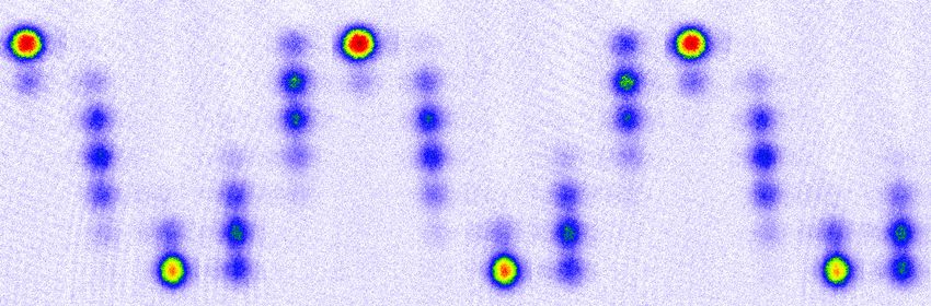
cally follows the slow change of the orientation of the quanti- In Figs. 3(a,b,c) we show the Larmor precession of mag-
zation axis. This means that the Mz component measured via netization along the elongated cold atom clouds for different
Stern-Gerlach imaging is equal to the My component at the expansion times T E . For short interrogation times T R , the
moment right before the second π/2 pulse is applied. mF -state populations collectively oscillate in time for all T E ,
In the presence of a strong magnetic field gradient of meaning hS y (x)i is almost independent of position x along the
100 G/cm, the atom cloud splits into separated clouds ac- cloud. However, for longer T R , the mF -state populations be-
cording to their mF -states [16–19]. After T S G = 10 ms of come space-dependent (Fig. 4). This is caused by the pres-
Stern-Gerlach splitting, we take a standard absorption image ence of the component ∂Bx /∂x of the magnetic field gradient.
of the separated clouds and calculate the expectation value of Fig. 4(b) shows the position dependent hS y (x)i for different
the spin z-component values of T R and is a signature measurement of the presented
P+3 magnetic gradiometer detection principle.
mF =−3 mF NmF Before we proceed with the evaluation of the component
hS z i = P+3 , (3)
mF =−3 NmF ∂Bx /∂x of the magnetic field gradient, we first analyse the
expansion of cold atom cloud in a dimple beam. The initial
where NmF is the atom number population in state mF . Simi- cloud widths σz0 and σ x0 are obtained from the analysis pre-
larly, we can calculate the variance of S z defined as sented in Figs. 3(d,e) by fitting the atom density profiles dur-
P+3 ing both free-space expansion and expansion along the dimple
mF =−3 m2F NmF beam. Notably, when σ x
σ x0 , which is after ∼ 20 ms of
h∆ S z i =
2
− hS z i2 . (4)
√ σ x starts increasing linearly in
P+3 expansion in a dimple beam,
mF =−3 NmF
time with a velocity v x = kB T x /m = 9.0 ± 0.1 mm/s, where
If the atoms are fully polarized and precess around the mag- kB and m are the Boltzmann constant and atomic mass of ce-
netic field perpendicular to their magnetization, the variance sium, respectively. This justifies a simple model of phase dif-
is equal to 0.5 when time averaged over one precession period ference accumulation in expanding atom cloud schematically
[17]. However, in the presence of decoherence, the time av- presented in Fig. 5.
erage of h∆2 S z i increases with the interrogation time T R . If For a nonexpanding cloud the phase difference ∆φstatic ac-
the elongated cloud is oriented along the x-direction, the z- cumulated during the interrogation time T R can be derived di-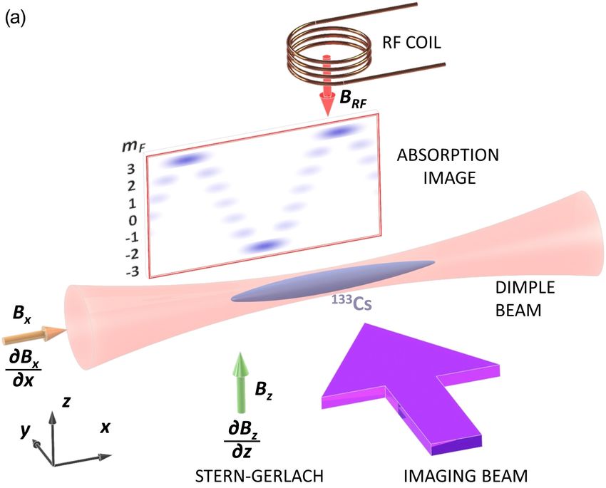
4
1.5
(a) TE = 0 ms, TSG = 10 ms
(a)
z (mm)
z (mm) 2
1.0 1
0.5 0
(b) TE = 20 ms, TSG = 10 ms
0.0
z (mm)
2
1
= 1905 Hz (b)
3 Rabi
0
Sx>
0 (c) TE = 40 ms, TSG = 10 ms
<
z (mm)
2
-3
1
0
0.0 0.2 0.4 0.6 0.8
t RF
(ms) 500
(d) (e)
1.5 (c) 150
400
z (mm)
1.0
300
m)
m)
0.5
100
3D TOF
(
(
0.0
z
x
200
= 49850 Hz
3 L
50
Sy>
0 100
<
1D TOF
-3
(d)
0 0
0 20 40 0 20 40
0 50 100 150 200
TR ( s)
tTOF (ms) tTOF (ms)
FIG. 2. (a) The Stern-Gerlach measurements showing separated FIG. 3. Larmor precession of mF -state populations for expansion
atom clouds corresponding to the different mF -state populations times (a) T E = 0 ms, (b) T E = 20 ms and (c) T E = 40 ms. Here the
ranging from mF = −3 (at the bottom) to mF = +3 (at the top). In interrogation time T R runs from 0 µs to 36 µs in steps of 4 µs (T S G =
the displayed absorption images the RF pulse length, tRF , increases 10 ms). The absorption images show the area of 1407 µm × 2110 µm.
from 528 µs to 788 µs in steps of 20 µs. (b) Oscillations of hS x i (d) The extracted 1/e widths σz as a function of time-of-flight (TOF)
as a function of tRF with νRabi = 1905 Hz (solid line). (c) Absorp- during free-space expansion (blue squares, 3D TOF) and expansion
tion images showing the Larmor precession of magnetization, where along a single dimple beam (red diamonds, 1D TOF). From the fit
the separation between two π/2 pulses, T R , increases from 12 µs to with the model σ2z = σ2z0 + kB T z /m · tT2 OF , σz0 = 12 ± 2 µm and
64 µs in steps of 4 µs. (d) Oscillations of hS y i as a function of T R T z = 1.27 ± 0.02 µK are obtained. (e) σ x for expansion along a
with νL = 49850 Hz (solid line). The red regions in (b) and (d) mark dimple beam (red circles) together with the corresponding fit (solid
the experimental points shown in (a) and (c), respectively. Each ab- line) using σ2x = σ2x0 + kB T x /m · tT2 OF . We obtain σ x0 = 69 ± 2 µm
sorption image in (a) and (c) shows the area of 376 µm × 1738 µm. and T x = 1.29 ± 0.02√µK. The dashed line follows the linear-in-time
In all these experiments T S G = 10 ms. expansion with v x = kB T x /m = 9.0 ± 0.1 mm/s. The red and green
areas mark, respectively, the typical interrogation and Stern-Gerlach
detection time intervals in our measurement protocol.
rectly from Eqs. (1) and (2)
∂Bx
∆φstatic (x) = γ xT R , (5) field at the position (x1 + x2 )/2 (for details please refer to
∂x
Fig. 5).
which is proportional to ∂Bx /∂x and T R . However, due to
the effect of cloud expansion it can be shown using a simple In Fig. 4(b) we show the fits of experimental hS y (x)i using
geometric consideration that the phase difference ∆φexpanding Eq. (2) for a range of interrogation times T R . From each fit
must be renormalized according to we obtain the wavelength λ of helical spatial dependence of
magnetization. From λ we then calculate the component of
T E − T R /2 the magnetic field gradient. For nonexpanding case,
∆φexpanding (x) = ∆φstatic (x) · . (6)
T E + TS G
∂Bx
!
The renormalization factor takes into account that during the 2π
= , (7)
interrogation time T R the atoms on average feel the magnetic ∂x static γT R λ5
(a) 2
z (mm)
1
0
TR = 16 s 1 ms 3 ms 5 ms 7 ms 15 ms
(b) 3
Sy(x)>
0
<
-3
0 500 0 500 0 500 0 500 0 500 0 500
x ( m)
FIG. 5. Schematic illustration of cold atom cloud expansion. At
(c) (e)
3
time t = 0, when the perpendicular dimple beam is turned off, the
Bx/ x (mG/cm)
0
2 10 cloud starts expanding along the remaining dimple beam. At t1 , the
S
1 7.3 mG/cm
first π/2-pulse is applied and the magnetization starts precessing. At
t2 , the second π/2-pulse is applied and the Stern-Gerlach protocol
0
starts (green area), ending at t3 , when the absorption image is taken.
Sy(x)>
4 5 The red area marks the time interval in which the position-dependent
phase difference ∆φ(x) is accumulated. The atoms at the final posi-
2
static tion x3 reflect the average magnetic field between positions x1 and
0 (d) expanding x2 . Because the magnetic field is linearly dependent on the position
<
0 this is equal to the magnetic field at (x1 + x2 )/2. The correspond-
0 10 0 5 10 15 ing time is exactly in the middle of the interrogation time interval at
TR (ms) TR (ms) (t1 + t2 )/2 = T E − T R /2. The renormalization factor in Eq. (6) fol-
lows directly from similar triangles: (x1 + x2 )/2 : x3 = (T E − T R /2) :
(T E + T S G ).
FIG. 4. (a) Absorption images of position dependent mF -state popu-
lations for a range of interrogation times T R . The first image serves
as a reference; it is taken with a short T R = 16 µs and shows position-
independent populations of mF -states. The absorption images show
the area of 914 µm × 2110 µm (T E = 30 ms and T S G = 10 ms). (b)
Extracted hS y (x)i as a function of position x for different T R . (c) The
amplitude S 0 of the position dependent hS y (x)i obtained from sinu-
soidal function fits (red lines in (b)). (d) The variance h∆2 S y i, time
averaged over one precession period. (e) The extracted component
∂Bx /∂x of the magnetic field gradient for two scenarios: (i) the static the extracted values become constant and their error decreases
model (Eq. (7), blue circles) and (ii) the model taking into account with increasing T R for T R ≤ 15 ms. For even longer T R the
the expansion of cold atom cloud (Eq. (8), red circles). The error amplitude S 0 of modulated hS y (x)i becomes substantially re-
bars denote a standard deviation of magnetic field gradient obtained duced (Fig. 4(c)). Additionally, its time averaged variance
from 10 repetitions. h∆2 S y i increases (Fig. 4(d)), meaning that the decoherence
of magnetization becomes important and reduces the sensor
accuracy. The reason behind this observation is mainly in
whereas for expanding cloud, our measurement protocol (Fig. 5), where longer T R brings
∂Bx T E + TS G the interrogation interval closer to the point where the effects
!
2π
= · . (8) of finite initial size of atom cloud become relevant. How-
∂x expanding γT R λ T E − T R /2
ever, these mainly affect the decoherence of magnetization,
The expression for the magnetic field gradient is independent but have only a very small impact on the evaluation of mag-
of the atom-cloud temperature and that is one of the key re- netic field gradient from Eq. (8). Even for T R = 15 ms the
sults of our work. estimated systematic correction is below 3%. Finally, for in-
The importance of taking into account the effect of expan- terrogation time T R = 7 ms we obtain ∂Bx /∂x = 7.3 mG/cm
sion is best seen in Fig. 4(e), where we plot and compare with an estimated error below ±0.2 mG/cm in a single shot.
∂Bx /∂x obtained from Eqs. (7) and (8). Whereas for the static The measured magnetic field gradient is of external origin,
model (no expansion) the values of ∂Bx /∂x decrease with in- most probably arising from ionic pumps surrounding our ex-
creasing interrogation time T R , for the expanding-cloud model perimental chamber.6
IV. DISCUSSION AND CONCLUSIONS satisfying the condition σ x
σ x0 . For example, this can be
achieved by decreasing the initial size σ x0 of the atom cloud
before releasing it into the dimple beam. Alternatively, one
Using the described single-shot Stern-Gerlach magnetic
could use more strongly elongated atom clouds before the first
gradiometer it is in principle possible to determine any com-
π/2 RF pulse is applied.
ponent of the complete magnetic-field-gradient tensor ∂Bi /∂ j,
By creating a non-expanding cold atom cloud in an elon-
with i, j = x, y, z. ∂Bi can be selected by the direction of B0
gated box-shaped potential, the cloud would become homo-
(in Fig. 1, this is Bx ), whereas ∂ j can be chosen by the ori-
geneous, meaning that the errors in hS y (x)i become compa-
entation of the elongated cold atom cloud. However, in order
rable along the cloud and the magnetic field gradient can be
for the sensor accuracy to be similar for all measured ∂Bi /∂ j
easily calculated directly from Eq. (7), describing the non-
components, the imaging should preferably be perpendicular
expanding (v x = 0) case. For example, this can be achieved
to the elongated cloud and BRF perpendicular to B0 (Fig. 1).
by loading the atoms from a broad dipole trap directly into a
The presented method has the potential for miniaturization us-
single dimple beam, which is at both ends truncated with two
ing atom chips [27, 28]. Such technology shortens the time
narrow 532 nm laser beams acting as repulsive barriers. How-
needed to prepare cold atoms and facilitates the integration
ever, in this approach atomic diffusion will be present during
of laser beams and magnetic coils for producing the neces-
the measurement protocol, which will substantially reduce the
sary magnetic fields. For our method it is important that BRF
coherence time and the sensitivity of the instrument. A pos-
and B0 are homogeneous. If sufficient homogeneity cannot
sible solution is to prepare the atoms at much lower tempera-
be achieved with integrated coils, external coils could be used
tures [15], which can be in principle achieved by evaporative
with an atom chip. This type of device could also easily be
cooling in such a box-shaped trap.
rotated in space to measure the magnetic-field gradients in an
In summary, we have demonstrated a simple and versatile
arbitrary direction.
method for measuring components of the magnetic field gradi-
While the sensitivity and the accuracy of our device are ent in a single shot with an estimated absolute accuracy below
comparable to or even surpass current proposals [5, 6], it lacks ±0.2 mG/cm (±20 nT/cm). This method can be adopted to the
temporal resolution. The Stern-Gerlach detection of magneti- majority of cold-atom setups with different atomic species,
zation is destructive and ∼ 13 s are required to prepare a new where it can serve as a quantitative characterization tool or
elongated cloud of cold cesium atoms for each measurement. for the cancellation of magnetic field gradients [4, 6, 31, 32].
Using 87 Rb, a much faster production of cold atoms is possi- We emphasize that the sensitivity of our magnetic gradiometer
ble and could reduce the temporal resolution well below 1 s. suffers neither from atomic diffusion nor from fluctuations or
For example, in an all-optical 87 Rb setup, rates on the order drifting of homogeneous magnetic field since only spatially-
of 107 cold atoms per second were reported [29]. In Ref. 30 dependent components of the magnetic field (the gradients
atom-chip technology was used to achieve an even higher rate and higher derivatives) contribute to the measured space mod-
of about 108 atoms per second. ulated magnetization along the elongated cold atom cloud. In
There are multiple ways to improve the sensitivity of the addition, the presented method has the potential for minia-
gradiometer presented here while retaining the same bene- turization and for further improvements of its sensitivity to
fits and working principles. The minimal measurable gradi- magnetic field gradients in a single shot.
ent is limited by the length of the cloud since the precision
of our method decreases for longer wavelengths λ. Therefore,
a longer cloud would allow measurement of smaller gradi- ACKNOWLEDGMENTS
ents. The other option is to use longer interrogation times T R .
This improves the precision because λ decreases for the same We thank Wojciech Gawlik, Alan Gregorovič, Matjaž
gradient. However, T R cannot be increased indefinitely, be- Gomilšek and Philipp Haslinger for their comments and dis-
cause the signal amplitude S 0 decreases due to decoherence. cussions. This work was supported by the Slovenian Research
It would immediately be possible to allow longer T R , if one Agency (research core fundings No. P1-0125 and No. P1-
extends the magnetization coherence time. This depends on 0099, and research project No. J2-8191).
[1] A. Grosz, M. J. Haji-Sheikh, and S. C. Mukhopadhyay, High L. E. Sadler, and D. M. Stamper-Kurn, Phys. Rev. Lett. 98,
Sensitivity Magnetometers (Springer International Publishing, 200801 (2007).
Switzerland, 2017). [6] M. Koschorreck, M. Napolitano, B. Dubost, and
[2] M. W. Mitchell and S. P. Alvarez, Rev. Mod. Phys. 92, 021001 M. W. Mitchell, Appl. Phys. Lett. 98, 074101 (2011).
(2020). [7] S. Franke-Arnold, M, Arndt and A. Zeilinger, J. Phys. B: At.
[3] H. B. Dang, A. C. Maloof, and M. V. Romalis, Appl. Phys. Lett. Mol. Opt. Phys. 34, 2527 (2001).
97, 151110 (2010). [8] G. Labeyrie, C. Miniatura, and R. Kaiser, Phys. Rev. A 64,
[4] K. Sycz, A. M. Wojciechowski, and W. Gawlik, Sci. Rep. 8, 033402 (2001).
2805 (2018). [9] M. Takeuchi, T. Takano, S. Ichihara, Y. Takasu, M. Kumakura,
[5] M. Vengalattore, J. M. Higbie, S. R. Leslie, J. Guzman, T. Yabuzaki, and Y. Takahashi, Appl. Phys. B. 83, 107 (2006).7
[10] M. Koschorreck, M. Napolitano, B. Dubost, and [21] M. Vengalattore, S. R. Leslie, J. Guzman, and D. M. Stamper-
M. W. Mitchell, Phys. Rev. Lett. 104, 093602 (2010). Kurn, Phys. Rev. Lett. 100, 170403 (2008).
[11] A. Wojciechowski, E. Corsini, J. Zachorowski, and W. Gawlik, [22] J. Kronjäger, C. Becker, P. Soltan-Panahi, K. Bongs, and
Phys. Rev. A 81, 053420 (2010). K. Sengstock, Phys. Rev. Lett. 105, 090402 (2010).
[12] N. Behbood, F. Martin Ciurana, G. Colangelo, M. Napolitano, [23] Y. Eto, H. Saito, and T. Hirano, Phys. Rev. Lett. 112, 185301
M. W. Mitchell, Appl. Phys. Lett. 102, 173504 (2013). (2014).
[13] O. Eliasson, R, Heck , J. S. Laustsen, M. Napolitano, R. Müller, [24] S. Palacios, S. Coop, P. Gomez, T. Vanderbruggen, Y. N. Mar-
M. G Bason, J. J. Arlt, and J. F. Sherson, J. Phys. B: At. Mol. tinez de Escobar, M. Jasperse, and M. W. Mitchell, New J. Phys.
Opt. Phys. 52, 075003 (2019). 20, 053008 (2018).
[14] Y. Cohen, K. Jedeja, S. Sula, M. Venturelli, C. Deans, L. Mar- [25] T. Mežnaršič, T. Arh, J. Brence, J. Pišljar, K. Gosar, Ž.
mugi, and F. Renzoni, Appl. Phys. Lett. 114, 073505 (2019). Gosar, R. Žitko, E. Zupanič, and P. Jeglič, Phys. Rev. A 99,
[15] J. M. Higbie, L. E. Sadler, S. Inouye, A. P. Chikkatur, 033625 (2019).
S. R. Leslie, K. L. Moore, V. Savalli, and D. M. Stamper-Kurn, [26] C. P. Slichter, Principles of Magnetic Resonance (Springer Ver-
Phys. Rev. Lett. 95, 050401 (2005). lag, Berlin, 1996).
[16] Y. Eto, S. Sekine, S. Hasegawa, M. Sadgrove, H. Saito, and [27] M. Keil, O. Amit, S. Zhou, D. Groswasser, Y. Japha, and R. Fol-
T. Hirano, Appl. Phys. Express 6, 052801 (2013). man, J. Modern Optics 63, 1840 (2016).
[17] Y. Eto, H. Ikeda, H. Suzuki, S. Hasegawa, Y. Tomiyama, [28] D. Becker et al., Nature 562, 391 (2018).
S. Sekine, M. Sadgrove, and T. Hirano, Phys. Rev. A 88, [29] T. Kinoshita, T. Wenger, and D. S. Weiss, Phys. Rev. A 71,
031602(R) (2013). 011602(R) (2005).
[18] M. Sadgrove, Y. Eto, S. Sekine, H. Suzuki, and T. Hirano, J. [30] J. Rudolph, W. Herr, C. Grzeschik, T. Sternke, A. Grote,
Phys. Soc. Jpn. 82, 094002 (2013). M, Popp, D. Becker, H. Müntinga, H. Ahlers, A. Peters,
[19] A. A. Wood, L. M. Bennie, A. Duong, M. Jasperse, C. Lämmerzahl, K. Sengstock, N. Gaaloul, W. Ertmer and
L. D. Turner, and R. P. Anderson, Phys. Rev. A 92, 053604 E. M. Rasel, New J. Phys. 17, 065001 (2015).
(2015). [31] C. J. Dedman, R. G. Dall, L. J. Byron, and A. G. Truscott, Rev.
[20] L. E. Sadler, J. M. Higbie, S. R. Leslie, M. Vengalattore and Sci. Instrum. 78, 024703 (2007).
D. M. Stamper-Kurn, Nature 443, 312 (2006). [32] A. Smith, B. E. Anderson, S. Chaudhury and P. S. Jessen, J.
Phys. B: At. Mol. Opt. Phys. 44, 205002 (2011).You can also read