No-Regret Caching via Online Mirror Descent - ECE ...
←
→
Page content transcription
If your browser does not render page correctly, please read the page content below
No-Regret Caching via Online Mirror Descent
                Tareq Si Salem                              Giovanni Neglia                          Stratis Ioannidis
         Université Côte d’Azur, Inria             Inria, Université Côte d’Azur            Northeastern University
        tareq.si-salem@inria.fr                    giovanni.neglia@inria.fr                   ioannidis@ece.neu.edu

   Abstract—We study an online caching problem in which                 In this paper, we extend and generalize the analysis of
requests can be served by a local cache to avoid retrieval costs     Paschos et al. in two different directions:
from a remote server. The cache can update its state after a
batch of requests and store an arbitrarily small fraction of each       1) We assume the cache can update its state after processing
content. We study no-regret algorithms based on Online Mirror              a batch of R ≥ 1 requests. This is of interest both in
Descent (OMD) strategies. We show that the choice of OMD                   high-demand settings, as well as in cases when updates
strategy depends on the request diversity present in a batch and           may only occur infrequently, because they are costly
that OMD caching policies may outperform traditional eviction-
                                                                           w.r.t. either computation or communication.
based policies.
                                                                        2) We consider a broad family of caching policies based
                      I. I NTRODUCTION                                     on online mirror descent (OMD); OGD can be seen as
                                                                           a special instance of this family.
   Caches are deployed at many different levels in computer
                                                                        Our contributions are summarized as follows. First,
                                                                                                                         √  we show
systems: from CPU hardware caches to operating system
memory caches, from application caches at clients to CDN             that caching policies based on OMD enjoy O             T regret.
caches deployed as physical servers in the network or as             Most importantly, we show that bounds for the regret crucially
cloud services like Amazon’s ElastiCache [1]. They aim to            depend on the diversity of the request process. In particular,
provide a faster service to the user and/or to reduce the            the regret depends on the diversity ratio R/h, where R is the
computation/communication load on other system elements,             size of the request batch, and h is the maximum multiplicity
like hard disks, content servers, etc.                               of a request in a given batch. We observe that OMD with
   Most prior work has assumed that caches serve requests            neg-entropy mirror map (OMDNE ) surmounts OGD in the
generated according to a stochastic process, ranging from the        high diversity regime, and it is overturned in the low diversity
simple, memory-less independent reference model [2] to more          regime.
complex models trying to capture temporal locality effects and          Second, all OMD algorithms include a gradient update
time-varying popularities (e.g., the shot-noise model [3]). An       followed by a projection to guarantee that the new solution is
alternative modeling approach is to consider the sequence of         in the feasible set (e.g., it does not violate the cache capacity
requests is generated by an adversary, and compare online            constraints). The projection is often the most computationally
caching policies to the optimal offline policy that views the        expensive step of the algorithm. We show that efficient poly-
sequence of requests in advance [4].                                 nomial algorithms exist both for OGD (slightly improving the
   Recently, Paschos et al. [5] proposed studying caching            algorithm in [5]) and for OMDNE .
as an online convex optimization (OCO) problem [6]. OCO                 The remainder of this paper is organized as follows. We
generalizes previous online problems like the experts prob-          introduce our model assumptions in Sect. II. We present OMD
lem [7], and has become widely influential in the learning           algorithms and quantify their regret and their computational
community [6], [8]. This framework considers an adversarial          complexity in Sect. III. Finally, numerical results are presented
setting, where the metric of interest is the regret, i.e., the       in Sect. IV.
difference between the costs incurred over a time horizon T by          The complete proofs are available in [10].
the algorithm and by the optimal offline static solution. Online
                                                                                       II. S YSTEM DESCRIPTION
algorithms whose regret grows sublinearly with T are called
no-regret algorithms, as their time-average regret becomes           Remote Service and Local Cache. We consider a system in
negligible for large T . Paschos et al. proposed a no-regret         which requests for files are served either remotely or by an
caching policy based on the classic online gradient descent          intermediate cache of finite capacity. A cache miss incurs a
method (OGD), under the assumption that (a) the cache can            file-dependent remote retrieval cost. This cost could be, e.g.,
store arbitrarily small fractions of each content (the so-called     an actual monetary cost for using the network infrastructure,
fractional setting), and (b) the cache state is updated after each   or a quality of service cost incurred due to fetching latency.
request. Bhattacharjee et al. [9] extended this work proving         Costs may vary, as each file may be stored at a different remote
tighter lower bounds for the regret and proposing new caching        location.
policies for the networked setting that do not require content          Our goal is to study online caching algorithms that attain
coding.                                                              sublinear regret. Formally, we consider a stream of requests for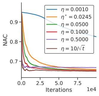
files of equal size from a catalog N = {1, 2, . . . , N }. These      each user for the additional delay to retrieve part of the file
requests can be served by a remote server at cost wi ∈ R+             from the server. Second, assuming that the R requests arrive
per request for file i ∈ N . We denote by w = [wi ]i∈N ∈ RN      +    and are served individually (e.g., because they are spread-out
the vector of costs and assume that w is known.                       within a timeslot), Eq. (3) can represent the load on the servers
   A local cache of finite capacity is placed in between the          or on the network to provide the missing part of the requested
source of requests and the remote server(s). The local cache’s        objects.
role is to reduce the costs incurred by satisfying requests           Online Caching Algorithms and Regret. Cache contents are
locally. We denote by k ∈ {1, . . . , N } the capacity of the         determined online: that is, the cache has selected a state xt ∈
cache. The cache is allowed to store arbitrary fractions of files,    X at the beginning of a time slot. The request batch rt arrives,
a common assumption in the literature [5], [11], [12] and a           and the linear cost frt (xt ) : X → R+ is incurred; the state
good approximation when the cache can store chunks of a file          is subsequently updated to xt+1 . Formally, the cache state is
and chunk sizes are much smaller than file size. We assume            determined by an online policy A, i.e., a sequence of mappings
                                                                              −1
that time is slotted, and denote by xt,i ∈ [0, 1] the fraction of     {At }Tt=1  , where for every t ≥ 1, At : (RR,h ×X )t → X maps
file i ∈ N stored in the cache at time slot t ∈ {1, 2, . . . , T }.   the sequence of the request batches and previous decisions
The cache state is then given by vector xt = [xt,i ]i∈N ∈ X ,         {(rs , xs )}ts=1 to the next state xt+1 ∈ X . We assume that the
where X is the capped simplex determined by the capacity              policy is initialized with a feasible state x1 ∈ X .
constraint, i.e.:                                                        We measure the performance of an online algorithm A
                    n             PN            o                     in terms of regret, i.e., the difference between the total
              X = x ∈ [0, 1]N : i=1 xi = k .                    (1)   cost experienced by a policy A over a time horizon T and
Requests. We assume that a batch of multiple requests may             that of the P   best static state x∗ in hindsight, i.e., x∗ =
                                                                                        T
arrive within a single time slot. Moreover, a file may be             arg minx∈X t=1 frt (x). Formally,
requested multiple times within a single time slot (e.g., by                                             ( T
                                                                                                          X               T
                                                                                                                          X
                                                                                                                                     )
different users, whose aggregated requests form the stream            RegretT (A) =           sup             frt (xt ) −   frt (x∗ ) ,
reaching the cache). We denote by rt,i ∈ N the number of                              {r1 ,...,rT }∈RT
                                                                                                     R,h   t=1          t=1
requests—also called multiplicity—for file i ∈ N at time t,                                                                         (4)
and by rt = [rt,i ]i∈N ∈ NN the vector of such requests,
                                                                      Note that, by taking the supremum in Eq. (4), we indeed mea-
representing the entire batch. We assume that the number of
                                                                      sure regret in the adversarial setting, i.e., against an adversary
requests (i.e., the batch size) at each timeslot is given by
                                                                      that potentially picks requests in RR,h trying to jeopardize
R ∈ N. We also assume that the maximum multiplicity of
                                                                      cache performance. In Sect. IV we show our caching policies
a file in a batch is bounded by h ∈ N. As a result, rt belongs
                                                                      performs well also under stochastic request processes and real
to set:
                   n                               o                  request traces.
                                      PN
          RR,h = r ∈ {0, . . . , h}N : i=1 ri = R .        (2)
                                                                             III. O NLINE M IRROR D ESCENT A LGORITHMS
   Intuitively, the ratio Rh defines the diversity of request            Upon seeing rt , the policy A could select as xt+1 the state
batches in a timeslot. For example, when R   h = 1, requests are      that would have minimized     (on hindsight) the aggregate cost
concentrated on a single content. When R
                                                                                         Pt
                                            h = N , requests are      up to time t (i.e., τ =1 frτ (x)). This can fail catastrophically,
spread evenly across the catalog N . For that reason, we refer        because of the adversarial nature of the requests. A more
to Rh as the diversity ratio. We note that our request model          conservative approach, that indeed leads to sublinear regret,
generalizes the setting by Paschos et al. [5] or Bhattacharjee        is to take gradient steps, moving in the direction of a better
et al. [9], which can be seen as the case R = h = 1 under             decision according to the latest cost. OMD denotes a family
our request model. We make no additional assumptions on               of gradient techniques.
the request arrival process; put differently, we operate in the          The main premise behind OMD [6, Sect. 5.3] is that
adversarial online setting, where a potential adversary may           variables and gradients live into two distinct spaces: the primal
select an arbitrary request sequence in RR,h to increase system       space, for variables, and the dual space, for gradients. The two
costs.                                                                are linked via a function known as a mirror map. Updates
Service Cost Objective. When a request batch rt arrives, the          using the gradient occur on the dual space; the mirror map
cache incurs the following cost:                                      is used to invert this update to a change on the primal
                           PN                                         variables. The standard online gradient descent OGD is a
                frt (xt ) = i=1 wi rt,i (1 − xt,i ).         (3)
                                                                      particular OMD algorithm where the mirror map is the squared
In other words, for each file i ∈ N , the system pays a cost          Euclidean distance. Other mirror maps may lead to better
proportional to the file fraction (1 − xt,i ) missing from the        performance depending on the specific problem [13, Section
local cache, weighted by the file cost wi and by the number           4.3].
of times rt,i file i is requested in the current batch rt .           OMD for Caching. Applied to our caching problem, both the
   The cost objective (3) captures several possible real-life         primal and dual spaces are RN . To disambiguate between the
settings. First, it can be interpreted as a QoS cost paid by          two, we denote primal points by x, y ∈ RN and dual points
by x̂, ŷ ∈ RN , respectively. Formally, OMD is parameterized Proof. Bubeck [13, Theorem 4.2] provides a general bound
by (a) a fixed learning rate η ∈ R+ , and (b) a differentiable on the regret of OMD, which in our caching setting becomes
map Φ : D → R, strictly convex over D and ρ-strongly convex η PT 2
RegretT (OMDΦ ) ≤ DΦ (xη∗ ,x1 ) + 2ρ t=1 k∇frt (xt )k∗
w.r.t. a norm k·k over X ∩D, where X is included in the closure
(11)
of D. The set X is the constraint set over which we optimize.
where k.k∗ is the dual norm of k.k, and x∗ is the best fixed
The function Φ is called the mirror map, that links the primal
decision in hindsight. The mirror map for OGD is Φ(x) =
to the dual space. Two additional technical assumptions on Φ 1 2
and D must hold. First, the gradient of Φ must diverge at the 2 kxk2 that is 1-strongly convex with regard to the Euclidean
norm (ρ = 1) and the dual norm is also the Euclidean one.
boundary of D. Second, the image of D under the gradient of
Let x1 be the minimizer of Φ(x), then we have
Φ should take all possible values, that is ∇Φ(D) = RN .
Given η and Φ, an OMD iteration proceeds as follows. After ∇ΦT (x1 )(x − x1 ) ≥ 0, ∀x ∈ X [6, Theorem 2.2] and,
observing the request batch rt and incurring the cost frt (xt ), from the definition of the Bregman divergence, DΦ (x∗ , x1 ) ≤
the current state xt is first mapped from the primal to the dual Φ(x∗ ) − Φ(x1 ).
The minimum value of Φ(x) over X is achieved when xi =
space via: k
N i ∈ N , and x∗ is an integral solution (i.e., k components
,
x̂t = ∇Φ(xt ). (5) of x∗ equal 1 and the others equal 0). Then Φ(x∗ ) = 21 k and
we get:
Then, a regular gradient descent step is performed in the dual 1
space to obtain an updated dual point: DΦ (x∗ , x1 ) ≤ k (1 − k/N ) (12)
2
ŷt+1 = x̂t − η∇frt (xt ). (6) We now bound the second term in (11). The maximum of krk2
is achieved when R h components are set to h, then:
This updated dual point is then mapped back to the primal √
space using the inverse of mapping ∇Φ, i.e.: max k∇fr (x)k2 ≤ max kwk∞ krk2 = kwk∞ Rh. (13)
r∈R r∈R
−1
yt+1 = (∇Φ) (ŷt+1 ). (7) Plugging
q (13) and (12) in (11), and selecting the learning rate
k
2
The resulting primal point yt+1 may lie outside the constraint η = k 1 − N /(kwk∞ hRT ), we obtain the upper bound
set X . To obtain the final feasible point xt+1 ∈ X , a projection in (10).
is made using the Bregman divergence associated with the
mirror map Φ; the final cache state becomes: The OGD Algorithm requires computing an Euclidean pro-
QΦ jection at each iteration, which, for general values of R and
xt+1 = X ∩D (yt+1 ), (8) h, can be performed in O N 2 steps using the projection
QΦ algorithm by Wang and Lu [14]. The algorithm proposed by
where X ∩D : RN → X is the Bregman projection defined as Paschos et al. [5], for the case R = h = 1, has O (N log(N ))
ΠΦX ∩D (y) = arg min DΦ (x, y). DΦ (x, y) = Φ(x) − Φ(y) − time-complexity, but we can achieve O (N ) complexity by
x∈X ∩D
T
∇Φ(y) (x − y) is the Bregman divergence associated with replacing the preliminary sorting operation with a O (log(N ))
the mirror map Φ. binary search and insertion.
A. Euclidean mirror map B. Neg-Entropy Mirror Map
1 2 We now consider a different mirror map, i.e., the neg-
The selection of the mirror map Φ(x) = 2 kxk2
and D =
RN yields the identity mapping ∇Φ(x) = x, for all x ∈ D. entropy mirror map, defined as follows:
Furthermore, the Bregman divergence associated with this map N
2
X
is just the Euclidean distance DΦ (x, y) = 12 kx − yk2 [13, Φ(x) = xi log (xi ) , and D = RN
>0 . (14)
Section 4.3]. Upon receiving a request batch rt , the algorithm i=1
updates its current state according to steps (5)-(8), this gives It can be checked that this map satisfies all requirements in
the OGD update rule: Sect. III., We refer to the OMD algorithm with the neg-entropy
xt+1 = ΠX (xt − η∇frt (xt )), ∀t ∈ {1, . . . , T − 1}, (9) mirror map as OMDNE .
We first characterize the regret of OMDNE :
where ΠX (·) is the Euclidean projection onto X . This setup of q
OMD coincides with OGD, studied by Paschos et al. [5]. We Theorem III.2. For η = 2kwk log(N/k)
2 2 , the regret of OMDNE
∞h T
present a new regret bound in Theorem III.1, that takes into satisfies:
account diversity, and improves over the √bound in [5] (valid p
RegretT (OMDNE ) ≤ kwk∞ hk 2 log(N/k)T . (15)
only for R = h = 1) by a factor at least 2.
r Proof. The proof is similar to the proof of Theorem III.1.
k(1− N
k
)
Theorem III.1. For η = 2
kwk hRT
the regret of OGD, The neg-entropy mirror map is ρ = k1 strongly convex w.r.t
∞
satisfies: the k.k1 over X [8, Example 2.5] and the corresponding dual
q norm is k·k∞ . Moving from (11), we bound the diameter of
k
RegretT (OGD) ≤ kwk∞ hRk 1 − N T (10) X w.r.t. to the Bregman divergence as well as the k·k∞ ofsteps per iteration. This results in an overall time complexity
Algorithm 1 Neg-Entropy Bregman projection onto X of O (N + k log(k)) per iteration of OMD, for general R, h
Require: N ; k; kyk1 ; P ; Sorted yN ≥ .. ≥ yN −k+1 ≥ yi , ∀i ≤ N − k values, and O (k) per iteration of OMD, when R = h = 1.
// y is the decision vector that lies outside of X .
// The scale P is a global variable initialized to 1. Proof. We adapt the Euclidean projection algorithm in [14].
1: yN +1 ← +∞
2: for b ∈ {N, . . . , N − k + 1} do Finding the projection x = ΠΦ X ∩D (y) corresponds to solving
3: mb ←
kyk − N
k+b−N
P
y P
i
a convex problem as DΦ (x, y) is convex in x and X ∩ D
1 i=b+1
4: if yb mb P < 1 ≤ yb+1 mb P then is a convex set. Without loss of generality, we assume the
// Appropriate b is found. components of x = ΠΦ
5: for i ≥ b+1 do X ∩D (y) to be in non-decreasing order.
6: yi ← m1 P
b
Let b ∈ N be the index of the largest component of x
7: end for smaller than 1. The KKT conditions lead to conclude that
8: P ← mb P
9: return yP // yP is the result of the projection. if the components of y are ordered in ascending order, so
10: end if are the components of x, and it holds yb eγ < 1 ≤ yb+1 eγ ,
11: end for
where γ is the Lagrangian multiplier associated with the
capacity constraint. The value of b can be found by checking
gradients ∇frt (xt ). Finally, selecting this condition for the possible values of b. We observe that
q the learning rate that necessarily b ∈ {N − k + 1, . . . , NP
}. In fact, we cannot have
2
gives the tightest upper bound η = 2 log( N 2
k )/(kwk∞ h T ),
N
b ≤ N − k. If b ≤ N − k, we get i=N −k+1 xi ≥ k and the
we obtain the desired regret upper bound. capacity constraint implies that xi = 0, ∀i ≤ b, but we must
N
The following theorem characterizes under which diversity have xi > 0 since x ∈ X ∩ D and D = R>0 . As b > N − k,
regime OMDNE outperforms OGD, and contrariwise the then we only require the largest k components of y to perform
regime where OGD surmounts. the projection.
For a given b let:
Theorem III.3. OMD
√ NE has a tighter regret bound than k+b−N k+b−N
OGD when R h > 2 N k, while OGD has a tighter regret
mb := eγ = P b = kyk1 − N
P (17)
i=1 yi i=b+1 yi
bound than OMDNE when Rh < 2k.
The projection corresponds to setting map the components
The result is obtained by relaxing the regret bound in Eq. (15) yb+1 , . . . , yN to 1 and multiply the other N −b components by
using a sharp upper bound [15], which is subsequently com- mb . In order to avoid updating all components at each step, we
pared to Eq. (10), and the second regime is shown by using can simply set the components xi , i > b (those that should be
x
the lower bound log(1 + x) ≥ x+1 for x > −1. set equal to 1) to m1b . Then, at any time t, we can recover the
Theorem III.3 immediately implies the advantage of Qt
value of xt,i by P = i=1 mb,i , where mb,t is the returned
OMDNE over OGD in the high-diversity ratio regime, and mb from the Bregman projection at time step t. Then at any
it is overturned in the low-diversity regime. time step, the actual value of the decision variable is xP .
Beyond its improved performance in terms of regret the For general values of R and h, the projection step takes
neg-entropy mirror map comes with an additional computa- O (k) steps per iteration and a partial sort is required to
tional advantage: its projection step admits a highly efficient maintain top-k components of yt sorted; this can be done
implementation.
As ∂Φ(x)
∂xi =
1+log xi , the inverse mapping is using partial sorting in O (N + k log(k)) [16].
−1
given by (∇Φ) (ŷt+1 ) = exp(ŷt,i − 1). Hence, the map When R = h = 1, Alg. 1 leads to only a single state
i
to the dual space and back in Eqs. (5)–(7) can be concisely coordinate update, and requires O (log(k)) steps to maintain
written as: top-k components of xt sorted online.
∂frt (xt )
−η
yt+1,i = xt,i e ∂xi
, for all i ∈ N . (16)
Theorem III.4 implies that OMDNE has a much smaller
In other words, OMD under the neg-entropy adapts the cache computational cost than OGD. In fact, for general value of
state via a multiplicative rule, as opposed to the additive rule R and h, OMDNE requires O (N + k log(k)) operations per
of OGD. iteration, while OGD requires O N 2 operations. When R =
Finally, the projection algorithm onto the capped simplex h = 1, the overall time complexity is O (k) per iteration for
can be implemented in O (N + k log(k)) time for arbitrary OMDNE and O (N ) for OGD.
R, h using the waterfilling-like Algorithm 1. The algorithm
receives as input the largest k components of y sorted in a IV. N UMERICAL E XPERIMENTS
descending order. It then re-scales the b largest components A. Experimental setup
and N − b smallest ones by different constant factors; the
1) Datasets: Throughout all experiments, we assume equal
value of b is determined via a linear search. The following
costs per file, i.e., wi = wi0 = 1, ∀i ∈ N .
theorem holds:
Synthetic traces We generate synthetic datasets, as summa-
Theorem III.4. Algorithm 1 returns the projection ΠΦ
X ∩D (y) rized in Table I. Individual file requests are i.i.d. and sampled
under the neg-entropy Φ, onto the capped simplex X in O (k) from a catalog of N files according to a Zipf distributionTABLE I: Trace Summary
Trace # Batches T N R h α
Fixed Popularity 105 105 200 1 1 0.8
Batched Fixed Popularity (1) 104 104 200 5 × 10³ 40 0.1
Batched Fixed Popularity (2) 104 104 200 5 × 10³ 53 0.2
Batched Fixed Popularity (3) 104 104 200 5 × 10³ 346 0.7
Partial Popularity Change (1) 5 × 10³ 103 500 5 × 10³ 40 0.1
Partial Popularity Change (2) 5 × 10³ 103 500 5 × 10³ 169 0.4
Partial Popularity Change (3) 5 × 10³ 103 500 5 × 10³ 473 0.7
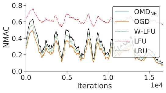
Akamai Trace 1.7 × 10⁴ 102 103 5 × 10³ 380 n/a (a) NAC of OGD (b) NAC of OMDNE (c) Time-Average Re-
gret
with exponent α. As we increase the exponent α, the requests Fig. 1: NAC of OGD (a) and OMDNE (b). Subfigure (c) compares
become more concentrated. Table I shows the value of h their TAC. The cache capacity is k = 10, and α = 0.8.
observed in each trace. The requests are grouped into batches
of size R, and η ∗ denotes the learning rate value specified in
Theorem III.1 and in Theorem III.2 for OGD and OMDNE , Finally, we consider the Time Average Regret TAR(A) ∈
respectively. [0, R], which is precisely the time average regret over the first t
We also generate non-stationary request traces (Partial time slots.
Popularity Change traces), where the popularity of a subset P
t Pt
of files is modified every T = 103 time slots. In particular TAR(A) = 1t s=1 fr s (xs ) − s=1 fr s
(x ∗ ) (20)
the 5% most popular files become the 5% least popular ones B. Results
and vice versa. We want to model a situation where the cache
knows the timescale over which the request process changes 1) Stationary Requests: Figures 1 (a) and 1 (b) show the
and which files are affected (but not how their popularity performance w.r.t. NAC of OGD and OMDNE , respectively,
changes). Correspondingly, the time horizon is also set to T under different learning rates η on the Fixed Popularity trace.
and, at the end of each time horizon, the cache redistributes We observe that both algorithms converge slower under small
uniformly the cache space currently allocated by those files. learning rates, but reach a final lower cost, while larger
The cache size is k = 5. learning rates lead to faster convergence, albeit to higher final
Akamai Trace We consider also a real file request from a cost. This may motivate the adoption of a diminishing learning
the Akamai CDN provider [17]. The trace spans 1 week, and rate, that combines the best of the two options, starting large
we extract from it about 8.5 × 10⁷ requests for the N = 103 to enable fast convergence, and enabling eventual fine-tuning.
most popular files. We group requests in batches of size R = We show one curve corresponding to a diminishing learning
5 × 10³ , and we consider a time horizon T = 100 time slots rate both for OGD and OMDNE , and indeed they achieve the
corresponding roughly to 1 hour. The cache size is k = 25. smallest costs. The learning rate denoted by η ∗ is the learning
2) Online Algorithms: In addition to the gradient based rate that gives the tightest worst-case regrets for OGD and
algorithms, we implemented three caching eviction policies: OMDNE , as stated in Theorems III.1 and III.2). While this
LRU, LFU, and W-LFU. LRU and LFU evict the least recently learning rate is selected to protect against any (adversarial)
used and least frequently used, respectively. W-LFU [18] is an request sequence, it is not too pessimistic: Figures 1 (a) and
LFU variant that only considers the most requested contents 1(b) show it performs well when compared to other learning
during a recent time window W , which we set equal to T × R rates.
in our experiments. The policies LRU, LFU, and W-LFU are Figure 1 (c) shows the time-average regret TAR of OGD
allowed to update the cache state after each request. Finally, and OMDNE over the Fixed Popularity trace. As both algo-
we define Best Static to be the optimal static allocation x∗ . rithms have sub-linear regret, their time average regret goes
We also define Best Dynamic to be the cache that stores the to 0 for T → ∞. Note how instead LRU exhibits a constant
k most popular files at any time for the synthetic traces (for time average regret.
which the instantaneous popularity is well defined). 2) Effect of Diversity: Figure 2 shows the NAC perfor-
3) Performance Metrics: We measure performance mance of OMDNE and OGD on the traces Batched Fixed
w.r.t. three metrics, that we define here. The Normalized Popularity (1), (2), and (3) under different cache capacities k
Average Cost NAC(A) ∈ [0, 1] corresponds to the time- and exponent values α. We observe that OMDNE outperforms
average cost over the first t time slots, normalized by the OGD in the more diverse regimes (α ∈ {0.1, 0.2}). This is
batch size R. more apparent for smaller values of k. In contrast, OGD out-
Pt performs OMDNE when requests are less diverse (α = 0.7);
1
NAC(A) = Rt s=0 frs (xs ) (18) again, this is more apparent for larger k. These observations
agree with Theorems III.3, which postulated that high diversity
The Normalized Moving Average Cost NMAC(A) ∈ [0, 1]
favors OMDNE .
is computed similarly using a moving average instead over a
3) Robustness to Transient Requests: Figure 3 shows the
time window τ > 0 (we use τ = 500 in our experiments):
Pt normalized average cost of OMDNE and OGD over the Partial
1
NMAC(A) = R min(τ,t) s=t−min(τ,t) frs (xs ) (19) Popularity Change traces, evaluated under different diversity(a) k = 2, α = 0.1 (b) k = 5, α = 0.1 (c) k = 10, α =
0.1 Fig. 4: NMAC of the different caching policies evaluated on the
Akamai Trace.
is that OGD is favourable in low-diversity regimes, while
OMDNE outperforms OGD under high diversity. Our prelim-
(d) k = 2, α = 0.2 (e) k = 5, α = 0.2 (f) k = 10, α = inary evaluation results also suggest that gradient algorithms
0.2 outperform classic eviction-based policies. We plan to conduct
a more thorough comparison as future research.
Acknowledgement. G. Neglia and S. Ioannidis acknowledge
support from Inria under the exploratory action MAMMALS
and the National Science Foundation (NeTS:1718355), respec-
tively.
(g) k = 2, α = 0.7 (h) k = 5, α = 0.7 (i) k = 10, α = R EFERENCES
0.7
[1] AWS, “Amazon Web Service ElastiCache,” 2018. [Online]. Available:
Fig. 2: NAC of OMDNE and OGD evaluated under different cache https://aws.amazon.com/elasticache/
sizes and diversity regimes. [2] E. G. Coffman and P. J. Denning, Operating systems theory. Prentice-
Hall Englewood Cliffs, NJ, 1973, vol. 973.
[3] S. Traverso et al., “Temporal Locality in Today’s Content Caching: Why
It Matters and How to Model It,” SIGCOMM Comput. Commun. Rev.,
vol. 43, no. 5, pp. 5–12, Nov. 2013.
[4] A. Fiat, R. M. Karp, M. Luby, L. A. McGeoch, D. D. Sleator, and N. E.
Young, “Competitive paging algorithms,” Journal of Algorithms, vol. 12,
no. 4, pp. 685 – 699, 1991.
[5] G. S. Paschos, A. Destounis, L. Vigneri, and G. Iosifidis, “Learning to
cache with no regrets,” in IEEE INFOCOM 2019 - IEEE Conference on
(a) α = 0.1 (b) α = 0.4 (c) α = 0.7 Computer Communications, 2019, pp. 235–243.
[6] E. Hazan, “Introduction to online convex optimization,” Found. Trends
Fig. 3: NAC of OGD and OMDNE evaluated under different diversity Optim., vol. 2, no. 3–4, p. 157–325, Aug. 2016.
regimes when 10% of the files change popularity over time. [7] N. Littlestone and M. Warmuth, “The weighted majority algorithm,”
Information and Computation, vol. 108, no. 2, pp. 212 – 261, 1994.
[8] S. Shalev-Shwartz, “Online learning and online convex optimization,”
regimes. Dashed lines indicate the projected performance in Found. Trends Mach. Learn., vol. 4, no. 2, p. 107–194, Feb. 2012.
the stationary setting (if request popularties stay fixed). The di- [9] R. Bhattacharjee, S. Banerjee, and A. Sinha, “Fundamental limits on
versity regimes are selected to provide different performance: the regret of online network-caching,” Proc. ACM Meas. Anal. Comput.
Syst., vol. 4, no. 2, Jun. 2020.
in (a) OMDNE outperforms OGD, in (b) OMDNE has similar [10] T. Si Salem, G. Neglia, and S. Ioannidis, “No-regret caching via online
performance to OGD, and in (c) OMDNE performs worse than mirror descent,” arXiv:2101.12588, 2021.
OGD. [11] L. Maggi, L. Gkatzikis, G. Paschos, and J. Leguay, “Adapting caching
to audience retention rate,” Computer Communications, vol. 116, pp.
Across the different diversity regimes, we find the OMDNE 159–171, 2018.
is more robust to popularity changes. In (a) and (b) OMDNE [12] K. Shanmugam, N. Golrezaei, A. G. Dimakis, A. F. Molisch, and
outperforms OGD in the non-stationary popularity setting: we G. Caire, “Femtocaching: Wireless content delivery through distributed
caching helpers,” IEEE Transactions on Information Theory, vol. 59,
observe a wider performance gap as compared to the stationary no. 12, pp. 8402–8413, 2013.
setting. In (c), the algorithms exhibit similar performance. [13] S. Bubeck, “Convex optimization: Algorithms and complexity,” Found.
4) Akamai Trace: Figure 4 shows that the two gradient Trends Mach. Learn., vol. 8, no. 3–4, p. 231–357, Nov. 2015.
[14] W. Wang and C. Lu, “Projection onto the capped simplex,”
algorithms, OMDNE and OGD, perform similarly over the arXiv:1503.01002, 2015.
Akamai Trace w.r.t. NMAC (the curves almost overlap). LRU, [15] C. Chesneau and Y. J. Bagul, “New sharp bounds for the logarithmic
LFU, and W-LFU may update the cache state after each function,” Electronic Journal of Mathematical Analysis and Applica-
tions, vol. 8, no. 1, pp. 140–145, 2020.
request, while the gradient algorithms can only update the [16] R. Paredes and G. Navarro, “Optimal incremental sorting,” in 2006
cache after R = 5000 requests. Nevertheless, the gradient Proceedings of the Eighth Workshop on Algorithm Engineering and
algorithms consistently outperform the classic ones. Experiments (ALENEX). SIAM, 2006, pp. 171–182.
[17] G. Neglia, D. Carra, M. Feng, V. Janardhan, P. Michiardi, and
V. C ONCLUSIONS D. Tsigkari, “Access-time-aware cache algorithms,” ACM Trans. Model.
Perform. Eval. Comput. Syst., vol. 2, no. 4, Nov. 2017.
We studied no-regret caching algorithms based on OMD [18] G. Karakostas and D. N. Serpanos, “Exploitation of different types of lo-
with the neg-entropy mirror map. Our analysis indicates that cality for web caches,” in Proceedings ISCC 2002 Seventh International
Symposium on Computers and Communications, 2002, pp. 207–212.
batch diversity impacts regret performance; a key findingYou can also read