Dynamos in Planets & Stars - Sabine Stanley University of Toronto
←
→
Page content transcription
If your browser does not render page correctly, please read the page content below
Dynamos in Planets & Stars

                      Sabine Stanley
                      University of Toronto
OUTLINE
1.   Intro to planetary & stellar dynamos

2.   Dynamo theory basics
     •  MHD approximation
     •  Magnetic Induction Equation
     •  Magnetic Reynolds #
     •  Alfven Approximation
     •  Self-sustained dynamos

3.   Planetary & stellar dynamo models
     •   Mean field models
     •   Macroscopic models
     •   Parameter regimes
     •   Scaling laws
     •   Surveying the models out there

 My (not so) hidden agenda:
 • planetary & stellar dynamos aren’t so different from each other, making it
    surprising that researchers rarely work on both
 • very similar processes, just in different parameter regimes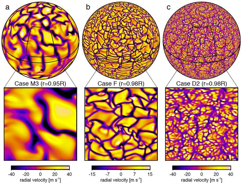
1. INTRO TO PLANETARY & STELLAR DYNAMOS
• convert mechanical energy into electromagnetic energy producing
  magnetic fields we can observe
                                                        complex
                                                        motions
                                                            +
                                                      electrically
                                                      conducting
                                                         fluid
                                                            +
                                                      presence
                                                        of a
                                                     magnetic field

                                                       maintain
                                                     field against
                                 (image courtesy
                                 NASA Goddard)
                                                     Ohmic decay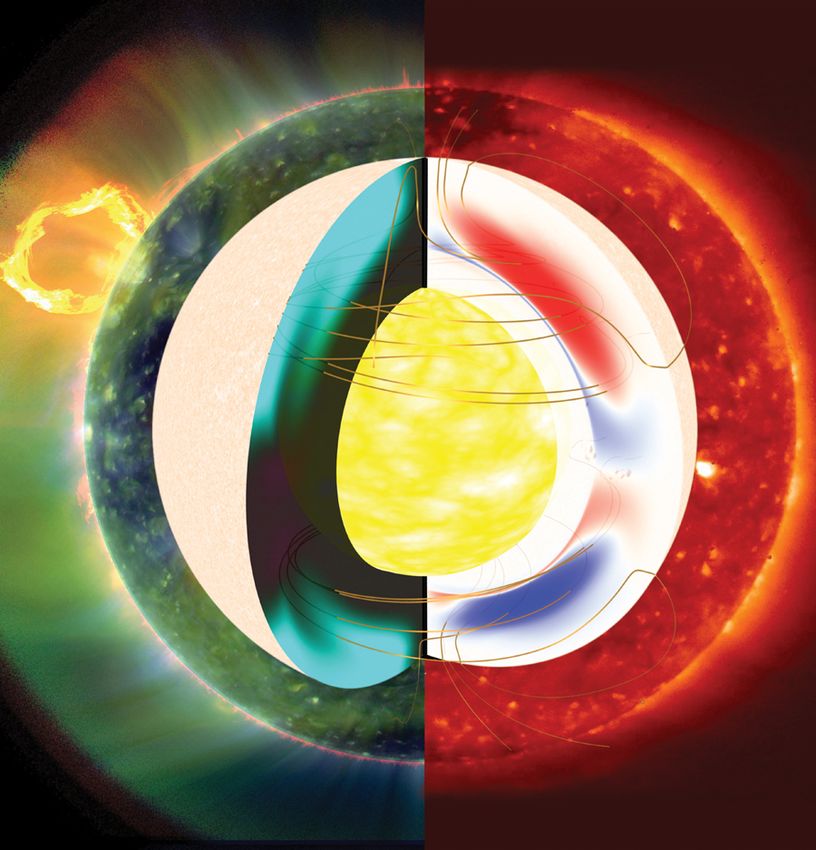
DYNAMO INGREDIENTS
        (1)electrically conducting fluid

        (2) fluid must have complex motions

        (3) motions must be vigorous enough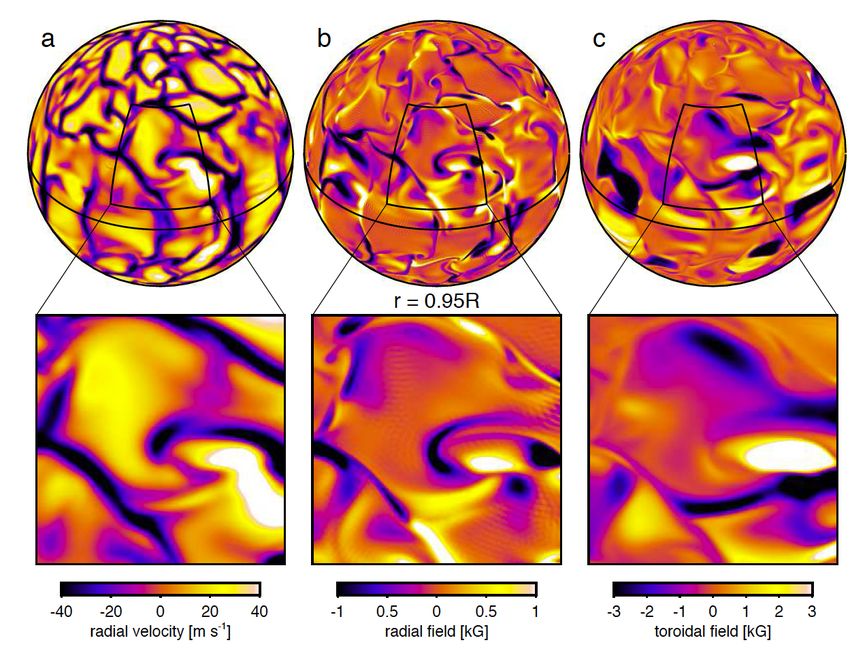
DYNAMO INGREDIENTS
        (1)electrically conducting fluid

           •   liquid iron (terrestrial planets)
           •   metallic hydrogen (gas giants)
           •   ionized water (ice giants)
           •   hydrogen plasma (stars)

        (2) fluid must have complex motions

           • lots of twisting, helical flows
           • rotation not required, but helpful
             in producing large-scale fields

        (3) motions must be vigorous enough

           • Velocity * Size * Conductivity
             must be big enough
           • The “magnetic Reynolds number
             condition” (see later…)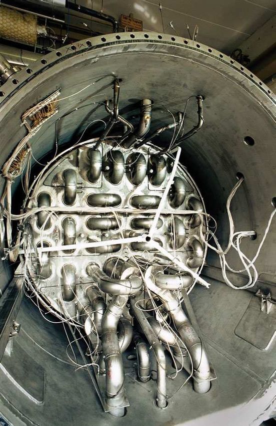
SOURCE OF COMPLEX MOTIONS
                      (1) Convection

                         • deep interiors: hot
                         • surfaces: cold
                         • if temperature difference large
                           enough: motions transport heat

                      (2) Shear

                         • causes magnetic fields to stretch
                         • good for magnetic field
                           generation

                      (3) Rotational Constraint

                         • rapid rotation organizes motions
                           in larger scales
    (image courtesy
    NASA Goddard)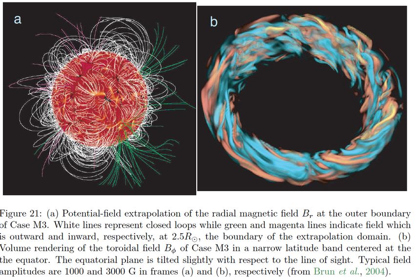
EARTH’S MAGNETIC FIELD
• We can only observe the field outside the surface.
• We try to infer what goes on in the dynamo source region

http://www.es.ucsc.edu/~glatz/index.html

• field in the source region               • observed field at the surface very
  likely very complicated                    dipolar

OBSERVATIONS
•Earth’s field at the core-mantle boundary (CMB):
    •at least 3.5 billion years old (paleomagnetism)
    •polarity reverses chaotically
    •variable on all time scales

    http://www.epm.geophys.ethz.ch/~cfinlay/gufm1.html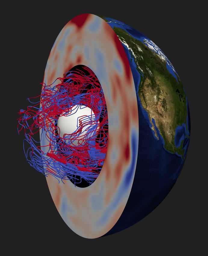
PLANETARY MAGNETIC FIELDS (ACTIVE)
                        nT
     Mercury
    Mercury                       Earth                      Jupiter

      Saturn                     Uranus                     Neptune

                             & Ganymede

• there are similarities & differences which are linked to interior properties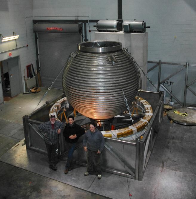
PLANETARY MAGNETIC FIELDS (PAST)
  Earth @ surface                                    Planetesimals & Asteroids?
      Maus (2010)

                                                                Weiss et al. (2008)

                            Mars @ 200km, from magnetometer
      Moon @ 30km           Langlais et al. (2004)

Richmond & Hood (2008)
SOLAR MAGNETIC FIELD • strong magnetic field associated with sunspots (~ 0.2 T or 2 kG) • global field of ~10-4 T or 1 G, approximately dipolar
SOLAR MAGNETIC FIELD

• field reverses polarity every ~ 11 years (“solar cycle”)
• solar cycle: sunspots appear at mid-latitudes, then region migrates toward
  equator. Then new group appears at mid-latitudes with flip of polarity
• sunspots have been continuously observed since time of Galileo
• Maunder minimum: time period (1647-1715) when sunspots were absent
CONVECTION ZONE & TACHOCLINE
• helioseismology tells us rotation profile in convection zone
• strong shear layer at base of convection zone may be very important for
  storing magnetic fields, producing cycles & spots
STELLAR MAGNETIC FIELDS
•   correlations between stellar types and
    magnetic field properties, probably due to
    geometry of convection zones

•   stars with outer convection zones (late-type
    stars) have observed magnetic fields whose
    strength tends to increase with their angular
    velocity

•   Cyclic variations are known to exist only for
    spectral types between G0 and K7).
EFFECT OF ROTATION
STUDYING MAGNETIC FIELDS
•   observations from spacecraft
    and telescopes                             SWARM

SOHO
STUDYING MAGNETIC FIELDS
• paleomagnetism: investigating magnetic fields frozen into rocks
Weiss et al. (2008)
Left: sample of Martian meteorite
ALH84001
Right: Squid microscope scan of
magnetic field in sample
Earth’s dipole moment vs. timeSTUDYING PLANETARY MAGNETIC FIELDS
• experiments: build your own dynamo!
Karlsruhe dynamo Maryland dynamo experimentSTUDYING PLANETARY MAGNETIC FIELDS
• computer simulations: have computers
solve the governing equations2. DYNAMO THEORY BASICS
• Start with the EM stuff:
Lorentz force: • combined electric and magnetic force/
volume
Ohm’s Law: • how charges respond (i.e. move therefore
(simplified) producing a current) to EM forcesMHD APPROXIMATION • Magneto-Hydro-Dynamic (MHD) approximation is an approximation made to Maxwell’s equations when velocities
MAGNETIC INDUCTION EQUATION
• We don’t normally work directly with all the EM equations. Instead, we use
  the Lorentz force in the momentum equation plus we derive an equation
  from the EM equations called the Magnetic Induction Equation (MIE).

• Here is how:

                 (assuming  constant  conductivity)

                                                                  continued…
MAGNETIC INDUCTION EQUATION CONT. • Notice that the equation has the form of a source/diffusion equation. The growth or decay of B (LHS) is governed by its creation through induction processes (1st term on RHS) and diffusion processes (2nd term on RHS)
WORKING WITH THE MIE
• Is a dynamo mechanism necessary for planets and stars?
• e.g. could Earth’s field today just be a remnant field created during formation?
• If the field is remnant, there is no regeneration process à u = 0. Plug into the MIE:
• How long does it take for a given field to decay? (i.e. the “magnetic diffusion time”)
• What do we use for L? For planetary cores, L is sometimes taken to be the radius of
the core “R”. Other times (the more appropriate choice), L is taken to be the length
scale of the slowest decaying eigenmode which is:
• Using:
à"
• if the Earth’s field was remnant, its e-folding time would be 15000 yrs, but
paleomag tells us B ~ constant for past 3.5 billion years à not a remnant field
• (for stars: 109 years, so its not so easy to dismiss a remnant field hypothesis)INTERPRETING THE MIE
• Using standard vector identity, can rearrange as:
• Using Gauss’ magnetism law and a bit of rearranging then gives:
• This has a nice physical interpretation:
• LHS: Rate of change of field moving with the fluid parcel
(i.e the Lagrangian derivative)
• RHS:
• 1st term: stretching of field lines due to gradients in velocity
• 2nd term: change in field due to compression/dilatation of fluid parcels
• 3rd term: diffusionMIE: THE MAGNETIC REYNOLDS NUMBER
• In order to generate a dynamo the driving force must be larger than the
dissipative force
driving force dissipative force
• The ratio of these two terms is called the magnetic Reynolds number:
• Notice that it increases with increasing U and L and as the conductivity increases.
• Rem must be larger than a critical value (~10) for dynamo action to occur
• Its very hard to generate laboratory dynamos b/c length scales so small. Its easy in
very large bodies.MIE: ALFVEN’S THEOREM
• planets and stars have large magnetic Reynolds number:
• In order to understand properties of MHD in high Rem flows, look at
extreme case: The limit as
• This limit can be interpreted as the perfectly conducting limit since as:
• In this case, the magnetic diffusivity à 0 so we can ignore the diffusion term in
the MIE
• Alfven’s theorem results in the following 3 facts about magnetic fields in this limit:
1. magnetic flux through a surface moving with the fluid is constant
2. magnetic flux tubes move with the fluid
3. if 2 material particles are on the same field line at time 0, then they remain
on that field line for all time t>0.
• For a fluid that is not perfectly conducting, the effects of diffusion permit the
field to slip through the fluid.
• Alfven’s theorem can also be used for dynamo processes whose time scales are
much shorter than the magnetic diffusion time at that length scaleMIE: ALFVEN’S THEOREM EXAMPLE
• Consider a perfect conductor and a constant vertical magnetic field:
and a simple horizontal shear flow: .
• Can solve for B from the MIE: (prove on problem set):
• Notice in this example, that the action of the flow on the original field generates
new field (in the x direction). BUT, we don’t regenerate the original field. This is not a
“self sustaining dynamo” (i.e. after we’ve started, if we remove the original field, the
total field decays).MIE: SELF SUSTAINING DYNAMO EXAMPLE
• Consider a good, but not perfect conductor, so Rem is large but finite.
• Diffusion is most effective where the gradients of B are large.
• In the following example, large gradients only occur in small regions, elsewhere,
Alfven’s theorem holds well.
• This example is known as the “Vainshtein-Zel’dovich rope dynamo”:
• Left with twice as
much field
• Could remove initial
‘seed’ field and the
flow would continue
to regenerate it à
Self-sustained dynamoFLUID FLOWS IN DYNAMOS
• force balances determine the fluid motions in dynamo regions
• notice that in the previous heuristic examples, the flows were all fairly
simple
• in stars & planets, the flow is very turbulent (i.e. lots of length and velocity
scales, large amount of disorganization)
• Usually we are interested in how these flows generate the large scale
magnetic fields that we see.
• 2 possible ways to proceed:
1. attempt to parameterize the effects of the small scale turbulence on
the large scales (“mean field models”)
2. ignore the small scales, only investigate the effects of the larger scale
flows on the dynamo (“macroscopic models”)
• Both of these methods are used and provide us with useful information.3. PLANETARY & STELLAR DYNAMO MODELS
• MEAN FIELD MODELS: Work described here mostly done by Steenbeck, Krause &
Radler (1966, etc) and Parker (1955).
• Setup: Assume turbulent velocity field of characteristic length scale l0 which is
much smaller than the length scale L associated with the mean magnetic field
B0
• Only consider statistical properties of the turbulent velocity and magnetic fields
(e.g. the mean of the flow or field)
• Define “mean” of flow or field as average of quantity over a box of size a where
l0MEAN FIELD MODELS
• Write the magnetic field and velocity as the sum of the mean and perturbations
about the mean:
(For now assume mean velocity is 0
and flow is incompressible)
• Plug these forms of B and u into the magnetic induction equation:
• Take the average of this equation over the box of length a to get the mean
magnetic induction equation… (will do on problem set). Result…MEAN FIELD MODELS
evolution of mean B generated by induction due to
perturbation fields u and b
• the induction term is usually referred to as an emf:
• now for the parameterization: on the problem set you will show that with certain
assumptions, the emf can be written in terms of the mean field B0:
• all of the info about the small scale stuff is parameterized by the choice of tensor
coefficients.
• various theories, wanted behavior can be implemented in the coefficients.MACROSCOPIC MODELS
• numerically solve the equations for the fluid motions, BUT, work with
modest parameter values such that the fluid motions are not very
turbulent and hence can be resolved directly
• this is probably a “better” approach for planets than for stars
because of the physical properties of the dynamo regions, i.e.
planets have Rem that can be reached in models
• to solve for the velocity and magnetic fields self-consistently, need
equations for:
• conservation of momentum
• conservation of mass
• conservation of energy
• MIEMACROSCOPIC MODELS
• Magnetic induction equation:
∂B
= ∇ × (u × B) + λ∇ B
2
∂t
• Conservation of mass:
∂ρ
+ ∇ ⋅( ρu) = 0
∂t
• Conservation of momentum:
⎛∂ ⎞ δρ
⎜⎝
∂t
+ u • ∇ ⎟⎠ u + 2 Ω × u = −∇P +
ρ
g + ν ∇ 2
u +
1
3
ν ∇(∇ ⋅
u) +( 1
ρµ0
∇ ×)B ×B
u : velocity g : gravity σ : electrical conductivity
Ω : rotation vector ν : coefficient of viscosity µ0: magnetic permeability
P : modified pressure B : magnetic field ρ : density
• Driving force (buoyancy due to gravity) due to thermal effects à need an
equation of state and an energy equation to complete the system:MACROSCOPIC MODELS
• Equation of state (EOS):
Planets: (linear relation) Stars: (linearized ideal-gas)
• Conservation of energy:
(Notes: could also be written in terms of entropy S using thermodynamic relations, I’ve also assume
constant thermal conductivity)
⎛ DT α T T DP ⎞ J 2
ρC P ⎜ − ⎟ = + τ :∇u + H + k∇ 2
T
⎝ Dt ρCP Dt ⎠ σ
C p : specific heat α T : coefficient of thermal expansion H : internal heat sources
T : temperature τ : deviatoric stress tensor J : current density
k : thermal conductivityNON-DIMENSIONAL EQUATIONS
• common in planetary dynamo models to non-dimensionalize the equations.
• e.g.: using “Boussinesq” approximation:
• Momentum: EP m (∂ t + v ⋅∇)v + ẑ × v = −∇P + J × B + RaTr + E∇ 2 v
−1
• Magnetic Induction:
2
(∂ t − ∇ ) B = ∇ × (v × B)
• Energy: (∂ t − Pm Pr −1∇ 2 )T = − v ⋅∇T + Q
€
• Mass: ∇⋅v = 0
Non-dimensional Numbers:
α g0 ΔTr0 ν
Rayleigh #: Ra ≡ Prandtl #: Pr ≡
2Ωη κ
ν ν
Ekman #: E ≡ Magnetic Prandtl #: Pm ≡
2Ωr02 η
€PLANETARY PARAMETER REGIME
Christensen et al. 2008
What can’t we do right:
• viscosity & thermal diffusivity too large compared to magnetic diffusivity
• rotation too slow, much less turbulent
Hope that if we are getting the force balances right, then models might be telling us
something about core dynamics
• scaling laws suggest this is happening (e.g. Christensen 2010)SOLAR PARAMETER REGIME
• much larger Reynolds number than planetary dynamos à extremely turbulent
• much larger magnetic Reynolds number than planetary dynamos à magnetic field
generation on extremely small scales
• Rossby number larger (rotation less important)PLANETARY & STELLAR MODELS Aside from the fact that we can’t numerically simulation the right parameter regime… Positives: Negatives: Planet models: Planet models: • magnetic Reynolds #: ~1000, can • reversal timescale ~ 500,000 years, time get to these values in models without for reversals to occur ~ 1000 years à mean field parameterizations can’t observe reversals in a human life • rotation acts to organize flow which span promotes large scale fields • can’t observe flows in dynamo region • solid rocks at surface record past • dynamo regions far removed from fields (at least some info like pole surface location and intensity). This is how we know reversal timescales Solar/stellar models: Solar/stellar models: • can study reversals in human lifetime • Rem ~ 109, cannot get these values • have observations of flows in without mean field parameterizations convection zone from • flow more turbulent helioseismology • physical properties vary significantly over • dynamo region is near the surface so convection zone we see smaller scales
SCALING LAWS
  •   although we don’t work in the appropriate parameter regime, can we use models
      to determine scaling laws and hence properties of planetary & stellar dynamos

  •   e.g.: magnetic energy scales with power available to drive dynamo:

                 dipolar fields                            nondipolar fields

Christensen (2010)
SCALING LAWS
• scaling laws derived from numerical models seem to work well for observations
Christensen (2010)
(energy density available to drive dynamo)SCALING LAWS
• e.g.: field dipolarity depends on rotation/inertia balance:
(local Rossby number)
Christensen (2010)MACROSCOPIC EARTH MODELS
Earth: • Able to reproduce main
field characteristics
Model" even though not
working in Earth-like
parameter regime:
•axial-dipole dominance
Observations" •surface field intensity
•reversals
•secular variation
•core surface flowPLANETARY MACROSCOPIC MODELS
• Can’t work at parameters for other planets either, but there are
some planetary features that we can get right, e.g.:
- core geometry
- force balances
- buoyancy sources
- external influences
• Explaining major differences between planetary magnetic fields is
possible by appealing to differences in these features
Mercury Earth UranusMERCURY
Observables a model should explain:
(1) WEAK intensity of the field
Br
g1 0 = -‐‑195 ±10 nT
(2) LARGE quadrupole
g20/g10 = 0.38
(3) SMALL tilt
dipole tilt < 1o
(Anderson et al. 2011)CONTESTANTS FOR MERCURY DYNAMO MODEL
Gomez-Perez & Solomon 2010,
Stanley et al. Heimpel et al. Gomez-Perez & Wicht 2010,
2005 2005
low σ
Christensen 2006, Vilim et al. 2010
Christensen & Wicht 2008
Manglik et al. 2010 Gomez-Perez et al., 2010MARS ANCIENT DYNAMO
•Why is the crustal field concentrated in the southern hemisphere
and correlated with the crustal dichotomy?
Acuna et al. (1999)SINGLE HEMISPHERE DYNAMO
x 106
A
• Crustal Dichotomy formation mechanism à thermal variations at CMB
1
Roberts & Zhong (2007) hemispheric CMB thermal variation
0
−1
x 10 4
C
1
“Single-hemisphere dynamo”
0
(Stanley et al., 2008)
−1
• Death of the Dynamo:
• subcritical dynamos: Kuang et al. (2008)
• impacts: Arkani-Hamed & Olson (2010)GAS GIANTS
Jupiter
Saturn
• large pressure range à radially
variable properties can be importantSURFACE ZONAL FLOWS
σ(r)&ρ(r) σ(r) Heimpel & Gomez-Perez 2011
Glatzmaier 2005, reviewed in
Stanley & Glatzmaier 2010)
Guervilly et al. 2011
instabilities of
narrow zonal jets
results in axially-
dipolar fieldsSATURN’S AXISYMMETRY
Cao et al. 2011: dipole tilt < 0.06 degrees
• Although dynamo models dominated by
axial dipole component, this level of
axisymmetry is not seen.
• Take non-‐‑axisymmetric field and
axisymmetrize it somehow between the
dynamo region and the surface
Helium rain-‐‑out layer
(Stevenson & Salpeter 1977)CONTESTANTS FOR SATURN DYNAMO MODEL
• Thick stably-stratified • Thin stably-stratified layer
layer ~ 0.4 core radii ~ 0.1 core radii +bdy
thermal variations
• Average dipole tilt:
1.5 degrees • Average dipole tilt:
0.8 degrees
(Christensen & Wicht 2008) (Stanley 2010)ICE GIANTS
Uranus Stanley & Bloxham 2004, 2006
• work in a geometry suggested by
low heat flow observations
NeptuneICE GIANTS
Gomez-Perez & Heimpel 2007
• zonal flow dynamos
Guervilly et al. 2011
• instabilities of wide zonal jets results
in non-dipolar non-axisymmetric
fields
• width of jets controls topology of
magnetic field (explains difference
of Jupiter & Neptune)EXTRASOLAR PLANET DYNAMOS
• Gas giants: magnetic fields in ionized atmospheric layers can affect flows
(Batygin et al., 2010, 2011, 2013, Perna et al. 2010, Rauscher & Menou, 2012,
2013)
• Ocean planets: small variations in interior properties can lead to large changes
in magnetic field (Tian & Stanley, 2013)
• Rocky planets: metallic mantles can shield strong fields from reaching surfaces
(Vilim et al., 2013)
Terrestrial planet structure
Ocean planet structureSOLAR DYNAMO MODELS
1. Mean field models: (velocity imposed):
• use differential rotation profile from helioseismology
• meridional (N-S) transport model
• mean field parameterization for small scales
2. Interface models:
• same as 1. plus also include tachocline (shear layer at base of convection zone)
3. Flux Transport models:
• same as 2. plus include large scale meridional (N-S) circulation to transport fields
from tachocline to surfaceSOLAR DYNAMO MODELS:
4. Macroscopic models:
e.g.: Anelastic Spherical Harmonic (ASH) code:
• uses realistic values for solar radius, luminosity and mean rotation rate
• reference state is based on 1D solar structure models
• upper boundary placed below photosphere (0.96-0.98 Rs)
• lower boundary: base of convection zone, but some simulations allow
penetration into the radiative interior
• This model tries to simulate solar convection properly and see what magnetic
fields you get out of it. Reproduces solar differential rotation profileMAGNETIC FIELDS IN MACROSCOPIC MODELS
SPOTS & CYCLES IN MACROSCOPIC MODELS
•   models don’t produce a tachocline region, but one can be added artificially
•   recent models starting to produce cycles:
STELLAR DYNAMO MODELS

    •    Convection zone geometry likely plays an important role

                                                     (G star)

•       In cooler stars, the convective envelope deepens as the surface temperature/mass
        decreases

    •   In hotter stars, the convective envelope disappears, but a convective core builds
        up as the surface temperature mass/effective temperature increases
FULLY CONVECTIVE STARS
• dynamos may be fundamentally different than solar-type
stars
• no tachocline to store fields resulting in interface dynamos
• many fully convective stars observed to have strong
chromospheric H-alpha emission & FeH line ratios, indicative
of strong magnetic fields
• unclear how dynamos in fully convective stars depend on
rotation rate
• Doppler imaging of rapidly rotating M-dwarfs reveals dark
patterns at low and moderate latitudes (star spots) (Barnes et
al. 2001).EARLY-TYPE STARS • magnetic fields may be trapped inside core à not observable Brun et al. (2005)
SUMMARY

•   lots of variety in planetary and stellar dynamos, but the
    fundamental principles, mechanisms and problems are similar
    (i.e. they are not so different)

•   models and observations suggest that magnetic fields depend
    strongly on dynamo region geometry, stratification, rotation
    and other properties

•   models seem to be on the right track, but we should be careful
    and vigilant because of the vast distance between model and
    planet/star parameters

                            Thank You
You can also read