Stroke Level Prediction through Pacman Game Data - EPFL
←
→
Page content transcription
If your browser does not render page correctly, please read the page content below
Stroke Level Prediction through Pacman Game Data

                                    Chapatte Mateo, Parchet Guillaume, Wilde Thomas
                                   Department of Computer Science, EPFL, Switzerland
                                    Mentor: Arzu Güneysu Özgür, Laboratory: CHILI

   Abstract—Predicting the stroke level of a patient with
Pacman game data could greatly improve the field of stroke
rehabilitation as it would highly reduce the time required to
estimate the patient’s FMA. Nevertheless, this task needs to
be accurate and explainable as it takes place in the medical
domain.
   During our research, we found out that smoothness and
velocity were important factors to predict the stroke level.
Although the prediction of our models was not accurate enough
to be used in medical area, this research shows that, even with a
small number of patients, we can still find out a nice estimator.
                                                                       Figure 1.     Gamified upper arm rehabilitation with tangible robots
                      I. I NTRODUCTION
                                                                                         II. M ODELS AND METHODS
   The Cellulo for rehabilitation project aims to provide
practical and intuitive gamified rehabilitation using tangible      A. Data Processing
robots as game agents and objects. Pacman is the first game            The work is based on three data-sets. The first two are
that was designed with this approach and it is used to              very small and contain the patient’s FMA sub-scores as
perform iterative upper arm exercises on patients recovering        well as additional information such as the date they were
from strokes (Figure 1). Upper arm rehabilitation mainly fo-        interned, their age, weight, etc... The main data-set contains
cuses on relearning lost or weakened functional movements           raw measurements taken at regular time interval during
that are crucial for daily life activities.                         each of the plays performed by the patients. It contains as
   The Fugl-Meyer Assessment (FMA) scale is an index                well information on the game configurations and some pre-
to assess the sensorimotor impairment of individuals who            computed features from previous analysis done in CHILI lab
experienced a stroke. It is widely used for clinical assess-        (those are detailed in the feature section). This data-set had
ment of motor function. The therapists in Sion care center          been previously been cleaned of the data points further than
(Switzerland) started to use the Pacman gamified rehabilita-        three standard deviations away from the mean.
tion and collect data on their patient’s plays. This displays          Still, the minDist feature1 contained 2.4% of missing
valuable information that might help to evaluate a FMA sub-         values so we interpolated the missing ones with their neigh-
score regrouping the ones related to upper extremities. This        bouring values (as minDist is fairly continuous).
observation leads to two major questionings.                           It is important to note that even though the raw data
   How well can we predict the FMA sub-score of a new               contains 229’473 samples, this only represents a total of
patient by comparing his plays with the ones of previous            145 games realized by the 10 studied patients during their
patients? Can we detect if, on a new game, a patient’s              rehabilitation.
evaluated abilities regress or improve? This second point              The kind of data points we will train on is an important
could be used as a first warning for the therapists to better       choice for the future results. The four main ways we found
spot if the patient’s rehabilitation is in progress.                and explored were the followings:
   The main challenge to answer these questions comes from             • Use complete games as data points. This captures full
the fact that we only have a low number of patients (10                   motions and the overall game performance but this only
patients in total, with 9 distinct FMA scores). Also, an                  yields 145 data points in total. Still, it can prove useful
important recurrent aspect of medical fields is that we need              to better visualise the data.
to be able to explain the results in simple terms.                     • Use sub-games. Each game can be split at each time
   Effective recovery process includes large volumes of                   the patient collects an apple (which is seen through the
repetitive exercises. Therefore, we might expect more data                field game_id). This allows to capture long motions
to be collected along with the new patients and they might
be used to further refine the models we present.                      1 minDist   value relates the difficulty to follow a linear trajectory
and performances as well as multiplying by five the                             points with different FMA were separable or not. This also
       number of data points.                                                          aimed to determine the features responsible for most of the
   •   Use time windows of 10 seconds. As each game lasts                              variance on our four different data-sets.
       exactly 3min the split is easy to perform and we can
       capture relevant motion features in this time interval. It
       yields a total of 2’458 data points.
   •   Use sub-motions windows. By looking at changes in
       axis directions, we can split the data into short sub-
       motions (where a sub-motion is the collection of data
       points going in the same axis directions). This yields
       16’700 data points which is way more than the other
       data-sets but these data points capture less information
       and might not be as relevant.
B. Features
   An important part of the project was to decide which
features we should compute and use to train our models.
Indeed, this choice might completely change the results as
some features can greatly explain the state of the patient.
For example, the jerk 2 is often used as a measure of the
non-smoothness of a movement.                                                          Figure 2. PCA visualization on the 4 different data-sets
   To find the best features, we decided to start by accessing                         A. Aggregated by sub-motion windows
the results of two related papers: "Quantitative assessment                            B. Aggregated by game_id windows.
                                                                                       C. Aggregated by 10 seconds time windows.
based on kinematic measures of functional impairments                                  D. Aggregated by full game windows.
during upper extremity movements: A review" from Ana de
                                                                                          The explanation of the axis of the four PCA instance give
los Reyes-Guzmán et al. and "Systematic Review on Kine-
                                                                                       homologous and very interpretative results. If we analyse the
matic Assessments of Upper Limb Movements After Stroke"
                                                                                       3 axis of the PCA based on the data aggregated by full game
from Anne Schwarz et al.. Those two studies performed a
                                                                                       session, we get that :
search to find all metrics used in kinematic assessment and
                                                                                       The first component explains 32.8% of the variance which
classified them.
                                                                                       is around half of the total explained variance, the second
   This assessment led to the identification of 24 features
                                                                                       component explains 22.8% of the variance whereas the third
we could compute. Twenty basic ones: for each data-point
                                                                                       component explains 12.7% of the variance.
window, its corresponding mean, maximum, minimum, me-
dian and standard deviation of its velocity, acceleration, jerk                          4 most important features coefficient in the feature space
and minDist. Four additional features were computed from                                 for the first principal component
the velocity over the given data-point window: the rest ratio,                           features       mean       std jerk     mean        median
number of velocity peaks, velocity mean maximum ratio and                                               acc                     jerk        jerk
Fourier Transform level3 . They aim to measure the smooth-                               coefficient 0.316         0.295        0.288       0.286
ness of a movement. Indeed, a higher Fourier Transform                                    Here we can see that this component really represents
level means higher frequencies and implies non-smoothness.                             the smoothness of the patient, because all those features are
This is complemented with the number of velocity peaks, the                            related to the second or third derivative of the position.
rest ratio4 and the velocity mean maximum ratio.                                         4 most important features coefficient in the feature space
   The elbow maximum angular velocity and the trunk                                      for the second principal component
displacement were additional relevant features we cannot                                 features       median     mean v       mean        rest ratio
calculate with the current measurement taken during the                                                 v                       max
patient’s plays.                                                                                                                ratio v
C. Data Exploration                                                                      coefficient 0.392         0.381        0.361       -0.286
   1) PCA: We used principal component analysis (PCA),                                    The second component represents the speed. We can see it
in order to get a sense of the data and see whether the data                           is mainly explained by the mean and the median of the speed
                                                                                       which is an indicator of an overall high speed. A high mean-
  2 jerk:   rate of change of the acceleration, third derivative of the position       max ratio is equivalent to an overall quite constant speed.
  3 threshold    below which 80% of the energy of the Fourier Transform                Finally, we can notice that it is inversely proportional to the
reside
   4 the rest ratio is the ratio between the time the patient is moving and the        rest ratio, therefore this axis represents a great control over
time the velocity is below a 20% threshold                                             the speed.

                                                                                   2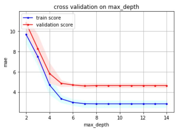
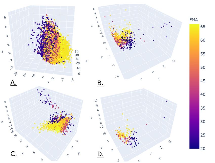
4 most important features coefficient in the feature space and a high mean jerk will be classified with a low FMA
for the third principal component score which is intuitive as a low velocity and non-smooth
features velocity mean std median movement can imply a bad quality of movements.
ft level minDist minDist minDist
coefficient 0.386 -0.381 -0.379 -0.340
X 12 ≤ -0.391
Lastly, the third component represents the minimal dis- gini = 0.551
samples = 560
value = [108, 110, 342]
tance to the linear trajectory and the velocity f t level. This True False
X 5 ≤ -0.039 X 5 ≤ 0.394
is interesting and also quite intuitive as the velocity f t level gini = 0.652
samples = 223
gini = 0.259
samples = 337
value = [78, 91, 54] value = [30, 19, 288]
is related to smoothness and the minDist value relates to a
difficulty to follow a linear trajectory. X 18 ≤ 1.888
gini = 0.577
gini = 0.064
samples = 60
gini = 0.149
samples = 301
X 8 ≤ 1.432
gini = 0.461
samples = 163 samples = 36
value = [20, 89, 54] value = [58, 2, 0] value = [6, 18, 277] value = [24, 1, 11]
2) OLS: We also ran an ordinary least square model
(OLS) on all our data-sets and they gave homologous results. X 10 ≤ -0.363
gini = 0.491
gini = 0.0 gini = 0.077 gini = 0.0
samples = 146 samples = 17 samples = 25 samples = 11
Let’s diagnose the OLS model run on the data aggregated value = [3, 89, 54] value = [17, 0, 0] value = [24, 1, 0] value = [0, 0, 11]
by full game session: X 22 ≤ -1.144 gini = 0.261
gini = 0.5
samples = 41
The R-squared is 0.888,it means that our features explain samples = 105
value = [0, 54, 51] value = [3, 35, 3]
about 89% of the variance which is an important amount X 8 ≤ -0.951
gini = 0.255
gini = 0.426
of the total variance. The adjusted R-squared is 0.866. Its samples = 40
value = [0, 34, 6]
samples = 65
value = [0, 20, 45]
closeness with the R-squared is an indicator that, overall,
gini = 0.346 gini = 0.223
the features are relevant. samples = 18
value = [0, 14, 4]
samples = 47
value = [0, 6, 41]
However, by looking at the t-statistic of each features
independently, we can notice that the majority of them do
not have a sufficient statistical significance. Furthermore, we Figure 3. Decision Tree with three FMA categories
noted that features related to extremes such as minimal or The two main metrics we used to analyse the results on the
maximal were the least significant. Therefore linear models test set were the mean absolute error (MAE) and the error
might perform poorly and we did not further explore such rate. The first one, gives us the average difference between
models. the true label and the prediction. The second one gives the
proportion of predictions that were further than a threshold
D. Models from their label. We found those two metrics interesting for
To answer our two questions, we decided to use two the project as they give a good interpretation of the results.
different techniques to learn our models: the Random Forest For both techniques cross validation was used to deter-
and the Decision Tree algorithm. We decide to keep the mine the best hyper-parameters. For the Random Forest, we
first one as it performs better than the Decision tree and saw that the n_estimator did not have a big impact on
as it can predict a FMA that is not in our data-set. This is the result once above 75. Indeed, beyond this threshold, the
useful because when we want to predict the FMA score of mean square error does not change much more (maximum
a new patient, we might not have his score in our data-set variation is 0.1 on validation). We decided to choose 100 as
(this is almost always the case for now as we only have 9 the default value of n_estimator as it had the best score
different scores) so we need to be able to predict new scores. for a relatively small number of trees, lowering the chance
The Decision Tree yields a lower general accuracy but it of over-fitting and the training time. The research of good
is way more explainable than the Random Forest. Indeed, hyper-parameters for the Decision Tree algorithm focused on
using the decision tree, we can explain step by step why the the ability for the tree not to over-fit too much the training
model chooses a score rather than another one based on the data. To achieve this we tuned the maximum depth parameter
evaluated features. as well as the minimum impurity decrease. In Figure 4, we
Figure 3 is an example of a decision tree trained at pre- can see that the mean squared error on the validation test
dicting one of three FMA categories (low [20,34], medium decreases until we reach 6 as maximum depth. With this
[35,49] or high [50,64] FMA). It shows each of its decisions information, the best trade-off seemed to use a maximum
and it is easy to interpret. In this example, to evaluate a new depth of 8 that would ensure enough power to the model as
data-point, the model will first look if the 12th feature (the well as limiting over-fitting.
median velocity) is below −0.391 or not. If it is the case,
it will go to the left and check weather the 5th feature (the III. R ESULTS
mean jerk) is below −0.039 or not. If not, it will go to the Our leave one out strategy proceeds as follows: one
right and, as a large majority of the previous data-points with participant is drawn out and the model is trained with
these characteristics were classified category 0 (low FMA), it the remaining participants, then we take the mean of the
will also classify this new data-point in category 0. From this predictions of the data points belonging to the participant
example we learn that someone with a low median velocity that was left aside. We repeat this for each participant
3would output as a prediction: the mean of the label of the
participants given for training. This model would output an
MAE of 18.1. In the random splitting strategy, the model
would output as a prediction: the mean of the label all the
participants. This model would output an MAE of 16.3.
In every setup, the data aggregated by sub-motion gives
the largest loss, this could come from the fact that by
aggregating in this way, we lose the information during the
change of direction which is probably relevant information.
We perform much better in random split; this is because
points coming from the same participant (and therefore same
FMA due to the small number of participants) tends to
cluster together. Overall, the loss is only a bit lower with
the decision tree. The scenario that will be the closest to a
Figure 4. Cross validation on max depth for Decision Tree (with 90% real-life application would be to classify a new participant,
bootstrapped confidence intervals with 1000 draws) therefore we would have a loss comparable to the "leave one
out" strategy. Because we want our model to be explainable
and finally we take the mean absolute error between each and that the decision tree does only perform bit worse
estimation and its real FMA label. than the random forest, we would choose the former and
In the random split, we split the data points into training aggregate our data by sub-games as it performs the best. This
(80%) and testing (20%), then aggregate the data points by score, 11.9, must be taken into perspective with 18.1 which
participants and take their mean as prediction. Finally, we is the upper bound above which our model is useless. Thus,
take the mean absolute error of this estimation and the real we can say our model is not great but perform reasonably
FMA label, for each participant. considering the amount of available data.
MAE loss on the random forest regressor5 .
IV. S UMMARY
different data aggregation
splitting game id game time sub- Predicting the FMA sub-scores related to upper extrem-
strategy session window motion ities using the Pacman data seems to be a promising tech-
(3min) (10s) window nique to help therapists to estimate their patient’s abilities.
Random 5.32 3.79 5.30 9.41 So far, the prediction of an unseen patient is still impre-
split cise, but it already gives a fair estimation and can underline
Leave 11.6 12.0 12.3 12.9 the aspects of his plays that led to the predicted FMA score.
one out
Additionally, the PCA visualisation yielded a better under-
MAE loss on the decision tree classifier6 . standing of the important characteristics a patient displays
different data aggregation while playing the Pacman games.
splitting game id game time sub- Overall, the results are encouraging if we take into ac-
strategy session window motion count the low number of patients and the model’s explain-
(3min) (10s) window ability that is required.
Random 5.24 4.69 5.48 11.38 To further improve the current models, we could try to
split prune some of the least useful features (for example with
Leave 11.9 12.2 12.1 14.6 a leave one out technique) and further prevent the trees
one out from over-fitting. One could also try to include features
specific to the patient’s characteristics such as their age (for
To have a comparison point, it is interesting to compute example, jerky movements might be more worrying for a
the MAE that would be achieved by a statistical model young patient).
that would not have access to the features of the data
points but would instead give a prediction that maximise
the likelihood. In the leave one out strategy, the model ACKNOWLEDGEMENTS
5 with n_estimator=100 The authors thank Arzu Güneysu Özgür and Chloé de
6 with min_impurity_decrease=0.01 and max_depth=8 Giacometti for their careful reading and helpful suggestions.
4R EFERENCES
[1] A. de los Reyes-Guzmán, I. Dimbwadyo-Terrer, F. Trincado-
Alonso, F. Monasterio-Huelin, D. Torricelli and A. Gil-Agudo,
"Quantitative assessment based on kinematic measures of func-
tional impairments during upper extremity movements: A re-
view," 2014, Clin Biomech (Bristol, Avon).
[2] A. Schwarz, CM. Kanzler, O. Lambercy, AR. Luftand and JM.
Veerbeek, "Systematic Review on Kinematic Assessments of
Upper Limb Movements After Stroke," 2019.
5You can also read