ATCOR Workflow for IMAGINE 2020 - Version 1.2.2 Step-by-Step Guide - GEOSYSTEMS
←
→
Page content transcription
If your browser does not render page correctly, please read the page content below
ATCOR Workflow for IMAGINE 2020
Version 1.2.2

Step-by-Step Guide

May 2020
ATCOR Workflow for IMAGINE Step-by-Step Guide Page 2/33
The ATCOR® trademark is owned by DLR
German Aerospace Center
D-82234 Wessling, Germany
URL: www.dlr.de
ERDAS IMAGINE® is a trademark owned by Hexagon AB.
The MODTRAN ® trademark is being used with the express permission of the owner, the United
States of America, as represented by the United States Air Force. While ATCOR uses AFRL's
MODTRAN code to calculate a database of LUTs, the correctness of the LUTs is the responsibility of
ATCOR. The use of MODTRAN for the derivation of the LUT's is licensed from the United States of
America under U.S. Patent No 5,315,513.
Implementation of ATCOR Algorithms
ReSe Applications Schläpfer
Langeggweg 3
CH-9500 Wil SG, Switzerland
URL: https://www.rese-apps.com
Integration in ERDAS IMAGINE, Distribution and Technical Support
GEOSYSTEMS GmbH
Gesellschaft für Vertrieb und Installation von Fernerkundungs- und Geoinformationssystemen mbH
Riesstrasse 10
D-82110 Germering
Phone: +49 - 89 / 89 43 43 – 0
Fax: +49 - 89 / 89 43 43 – 99
E-Mail: info@geosystems.de
Support: support@geosystems.de
URL: www.geosystems.de
Copyright © 2020 GEOSYSTEMS GmbH. All Rights Reserved.
All information in this documentation as well as the software to which it pertains, is proprietary material
of GEOSYSTEMS GmbH, and is subject to a GEOSYSTEMS license and non-disclosure agreement.
Neither the software nor the documentation may be reproduced in any manner without the prior written
permission of GEOSYSTEMS GmbH.
Specifications are subject to change without notice.
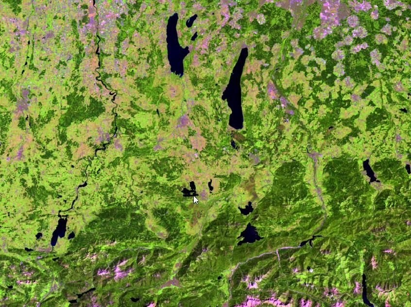
Cover: Sentinel-2, Netherlands, acquisition date: 5 August 2015, true color band composite;
top: original image, bottom: result of de-hazing with ATCOR Workflow for IMAGINE.
© GEOSYSTEMS GmbH, 2020
ATCOR Workflow for IMAGINE                                                          Step-by-Step Guide                                                              Page 3/33

Content
1            Overview .................................................................................................................................... 4
2            Example 1 .................................................................................................................................. 4
    2.1          What You Will Learn .............................................................................................................. 4
    2.2          Data Preparation .................................................................................................................... 5
    2.3          Data Processing Using the ATCOR Workflow Dialog ............................................................ 5
    2.4          Data Processing Using the ATCOR Workflow Operators ...................................................... 8
3            Example 2 ................................................................................................................................ 12
    3.1          What You Will Learn ............................................................................................................ 12
    3.2          Data Description ................................................................................................................... 12
     3.2.1       Landsat-5 TM Image ............................................................................................................................................ 12
     3.2.2       Digital Elevation Model ......................................................................................................................................... 13

    3.3          Data Processing Using the ATCOR Workflow Dialog .......................................................... 14
    3.4          Data Processing Using the ATCOR Workflow Operators .................................................... 19
4            Example 3 ................................................................................................................................ 24
    4.1          What you Will learn .............................................................................................................. 24
    4.2          Data processing Using the ATCOR Workflow Dialog .......................................................... 24
    4.3          Data processing Using the ATCOR Workflow Operators .................................................... 27
5            Appendix ................................................................................................................................. 32

© GEOSYSTEMS GmbH, 2020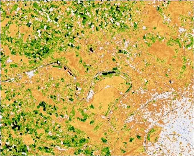
ATCOR Workflow for IMAGINE                            Step-by-Step Guide                              Page 4/33

1 Overview
This guide leads you through the major processing steps of ATCOR Workflow. All example data sets
are processed using both, the ATCOR Workflow Dialog and the ATCOR Workflow Operators
(Spatial Modeler).
Before you start, make sure that
              •    ERDAS IMAGINE Essential 2020 (for ATCOR Workflow Dialog) or ERDAS
                   IMAGINE Professional 2020 (for ATCOR Workflow Dialog and access to the ATCOR
                   Workflow operators) is installed and licensed,
              •    ATCOR Workflow for IMAGINE 2020 is installed and licensed, and that
              •    you have access to the internet for downloading the demo datasets
                   (Example 1: ~840 MB, Example 2: ~50 MB, Example 3: ~750 MB).
              •        ATCOR Workflow for IMAGINE is based on IDL (Interactive Data Language).
                   The free IDL Virtual Machine is included in the ATCOR Workflow Installer. With this
                   free IDL version, an IDL splash screen is displayed the first time an ATCOR
                   Workflow process in a session is run. Just click on the splash screen to remove it.
                   For disabling the splash screen (e.g. for unattended batch processing), an IDL
                   runtime license has to be purchased. If an IDL runtime license already exists,
                   ATCOR Workflow uses this license by default.

2 Example 1

2.1   What You Will Learn
Based on a Landsat-8 image (Figure 1 and 2), the following processing steps are demonstrated:
              •    automatic metadata import,
              •    haze reduction (ATCOR Dehaze), and
              •    atmospheric correction in flat terrain (ATCOR-2).
The example data set is processed using the ATCOR Workflow Dialog (Section 2.3) and the ATCOR
Workflow Operators (Spatial Modeler) (Section 2.4).

 Figure 1: Footprint of the Landsat-8 demo data set        Figure 2: True color quicklook of the Landsat-8 demo
 (Example 1), path/row: 199/026, date: 2013-04-14.         data set (after import in ERDAS IMAGINE).
                                                           [Image courtesy of the U.S. Geological Survey]

© GEOSYSTEMS GmbH, 2020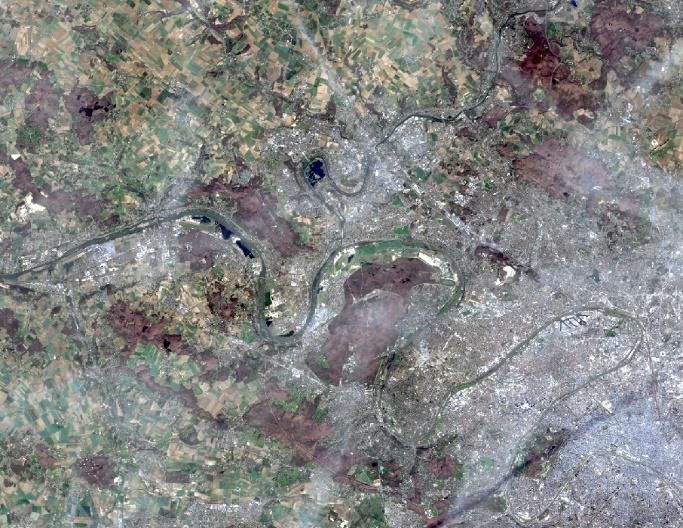
ATCOR Workflow for IMAGINE                          Step-by-Step Guide                               Page 5/33

2.2    Data Preparation
1.    Download the file ATCOR_Workflow_Step_by_Step_Guide_Example1.zip
      from http://www.geosystems.de/en/products/atcor-workflow-for-imagine/download and extract it
      to the folder \Example1\01_L8_data.

2.    Open the multispectral image by importing Bands 2,3 and 4 as Virtual Stack: File Tab > Open
      > Raster Layer…. Choose TIFF in the “Files of type” option and select
      LC81990262013104LGN01_B2.TIF, LC81990262013104LGN01_B3.TIF and
      LC81990262013104LGN01_B2.TIF.
      Navigate to the “Multiple” tab in the “Select Layer To Add:” dialogue and select “Virtual Stack”.
      Click OK. The virtual stack is opened in the 2D View window.
      Choose the band combination Layer 3 (red) - Layer 2 (green) - Layer 1 (blue) in the
      Multispectral Tab > Bands.

3.    Examine the multispectral image: The image (Figure 2) shows haze and cirrus clouds, so we
      will apply ATCOR Dehaze prior to atmospheric correction. As the area is rather flat, we will use
      ATCOR-2 for atmospheric correction. Additionally, we want to compute the LAI (Leaf Area Index)
      based on the Soil-adjusted Vegetation Index (SAVI).

2.3    Data Processing Using the ATCOR Workflow Dialog
1. Create the following folders (do not move the project data afterwards to other folders!):
         \Example1\02_atcor_project
         \Example1\03_output

2. Click Toolbox Tab > ATCOR Workflow for IMAGINE > Run ATCOR Dehaze to open the
   ATCOR Dehaze dialog.

3. Select the Operation Mode Create ATCOR Project.
4. Specify the following options on the Project Tab of the dialog (Figure 3):
              •    Project folder: navigate into the folder
                   \Example1\02_atcor_project
              •    Sensor: Landsat-8 MS + TIRS (10 Bands)
              •    Image File: switch off the file filter ‘All File-based Raster Formats’ by entering ‘*.txt’ in
                   the field ‘Image File’ and select the file
                   \Example1\01_L8_data\temp\
                   lc81990262013104lgn01\LC81990262013104LGN01_MTL.txt
              •    Metadata File: [no input required]

© GEOSYSTEMS GmbH, 2020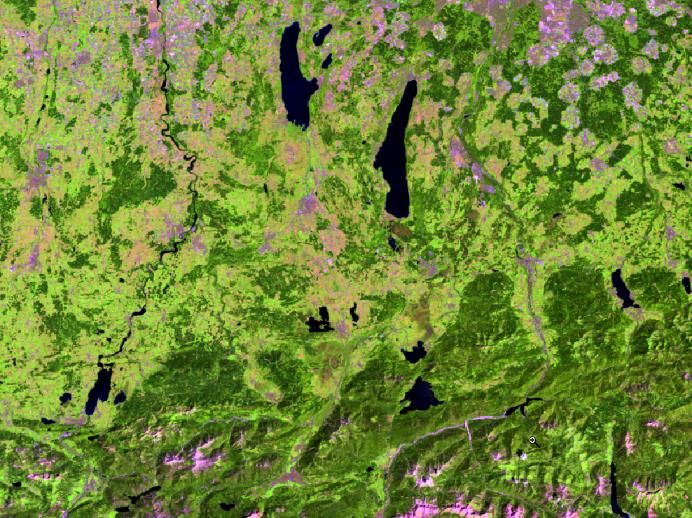
ATCOR Workflow for IMAGINE                        Step-by-Step Guide                               Page 6/33

              •   Elevation File: [no input required]
              •   Dehazed Image File: specify the name for the output file (new file)
                  \Example1\03_output\
                  LC81990262013104LGN01_dh.tif
5. Navigate from the Project Tab to the Settings Tab (Figure 4).
    The input values in the Sensor Information box and in the Geometry box will be set
    automatically for Landsat-8, as ATCOR Workflow provides metadata import for this sensor.
    Therefore, you do not have to edit these settings.
6. In the Dehaze Parameters box specify the following options:
              •   Dehaze Method:                        standard
              •   Dehaze Area:                          land pixels only
              •   Use Cirrus Band If Available:         ✓
              •   Interpolation Method:                 bilinear (fast)

 Figure 3: ATCOR Dehaze Project Tab.                        Figure 4: ATCOR Dehaze Settings Tab.

7. Click Run. Depending on your PC, processing can take about 5 minutes to finish. Check the
   process status in the ERDAS IMAGINE Process List.
8. Examine the Session Log. Here you find some basic information about the executed process as
   well as warnings or error messages if a problem occurred.
9. Examine the project folder:
   \Example1\02_atcor_project
    Here you find the following files:
              •   GEOSYSTEMS_ATCOR.project, the ATCOR project file, a text file containing some
                  basic information on the project,
              •   lc81990262013104lgn01.tif, the layer stack of the original image with the
                  band order and pixel size as required by ATCOR Workflow,
              •   lc81990262013104lgn01.log, the log file (during processing, ATCOR shows a
                  message that describes the required band order, within our example this can be
                  ignored), and
              •   lc81990262013104lgn01.cal, the calibration file.
10. Examine the log file. Here you can find detailed information about the executed process.
11. Open the original image and the dehazed image in the Viewer and compare (Figure 10).

© GEOSYSTEMS GmbH, 2020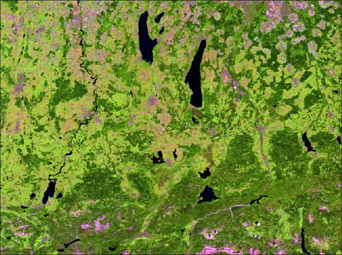
ATCOR Workflow for IMAGINE                         Step-by-Step Guide                        Page 7/33

    Original image: \Example1\02_atcor_project\
                    lc81990262013104lgn01.tif
    Dehazed image:\Example1\03_output\
                  LC81990262013104LGN01_dh.tif
    Now load the haze map into the viewer and compare with the original / dehazed image.
    Haze map:           \Example1\03_output\
                        LC81990262013104LGN01_haze_map.tif
Next, we atmospherically correct the dehazed image using the ATCOR-2 process.
12. Click Toolbox Tab > ATCOR Workflow for IMAGINE > Run ATCOR-2 to open the ATCOR-2
    dialog.

13. Select the Operation Mode Load ATCOR Project.
14. Specify the following options on the Project Tab of the dialog:
               •     Project Folder:
                     \Example1\02_atcor_project
               •     Corrected Image File: specify the name for the output file (new file)
                     \Example1\03_output\
                     LC81990262013104LGN01_atcor2.tif
15. Navigate from the Project Tab to the Basic Settings Tab (Figure 5).
    In the Sensor Information box and in the Geometry box the metadata values are shown as they
    were read from the metadata file, when the project was created. Do not edit these values!
16. In the Atmosphere box specify the following options after checking the corresponding Edit box:
           •       Water Vapor Category:         fall/spring
           •       Aerosol Type:                 rural
17. Navigate from the Basic Settings Tab to the Advanced Settings Tab (Figure 6). Check the
    checkbox Compute Value-added Products and select the LAI Model Use SAVI.
18. Click Run. Depending on your PC, processing can take about 5 minutes to finish. Check the
    process status in the ERDAS IMAGINE Process List.
19. Examine the Session Log (File Tab > Session > View Session Log). Here you can find basic
    information about the executed process as well as warnings or error messages if a problem
    occurred.
20. Examine the log file. Entries referring to the process ATCOR-2 were added to the file providing
    detailed information about the executed process.
21. Display the result and compare the atmospherically corrected image with the original image, e.g.
    by using the Inquire Curser. The corrected image provides surface reflectance spectra. You get

© GEOSYSTEMS GmbH, 2020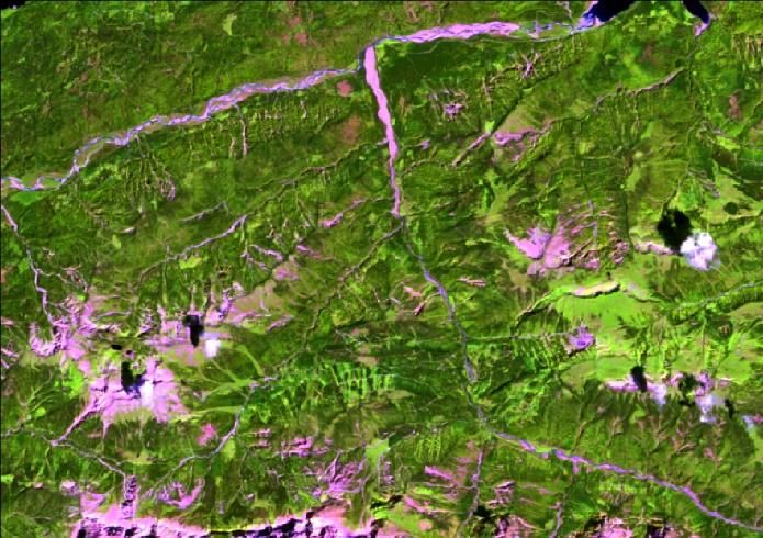
ATCOR Workflow for IMAGINE                          Step-by-Step Guide                             Page 8/33

      surface reflectance in % by dividing the pixel value by 100 (= applied reflectance scale factor). E.g.
      a pixel value of 2150 corresponds to a reflectance of 21.5%.

 Figure 5: ATCOR-2 Basic Settings Tab.                  Figure 6: ATCOR-2 Advanced Settings Tab.

2.4     Data Processing Using the ATCOR Workflow Operators
1. Create the following folders:
      \Example1\02_atcor_project_SM
      \Example1\03_output_SM

2. Click Toolbox Tab > Spatial Model Editor to open the Spatial Modeler.

Figure 7: ATCOR Workflow for IMAGINE button.
3. Navigate to the Operators window, open the group GEOSYSTEMS ATCOR, and add the
   operators Create ATCOR Project, Run ATCOR Dehaze, Set ATCOR Parameters, and Run

© GEOSYSTEMS GmbH, 2020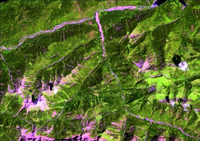
ATCOR Workflow for IMAGINE                       Step-by-Step Guide                             Page 9/33

    ATCOR-2 by drag-and-drop to the Spatial Model Editor. Connect the operators as shown in
    Figure 8.
4. Set the operator ports as follows (see also Figure 8) by double-clicking the corresponding ports:
    Create ATCOR Project:
             •    ATCORProjectFolder: navigate into the folder
                  \Example1\02_atcor_project_SM
             •    ImageFilename: switch off the file filter ‘All File-based Raster Formats’ by entering
                  ‘*.txt’ in the field ‘Image File’ and select the file
                  \Example1\01_L8_data\temp\
                  lc81990262013104lgn01\LC81990262013104LGN01_MTL.txt
             •    Sensor: Landsat-8 MS + TIRS (10 Bands)
    Run ATCOR Dehaze:
             •    DehazeMethod: standard
             •    DehazeArea: land and water pixels
             •    DehazedImageName:
                  \Example1\03_output_SM\
                  LC81990262013104LGN01_dh.tif
    Set ATCOR Parameters: Enable the ports by right-clicking the operator, select Properties. The
    Properties window is now located in the lower right corner of your screen. Enable the ports by
    checking the port in the ‘Show’ column. To set the port, double-click the port (not the operator) and
    select the following values:
             •    Water Vapor Category:        fall/spring
             •    Aerosol Type:                rural
             •    ValueAddedProds:             true

                     The computation of the value-added products file could also be enabled (not
                  recommended here!) by using the ‘Set ATCOR Parameters’ GUI that can be opened
                  by double-clicking the operator. The processing parameter Compute Value-added
                  Products is located on the Advanced Settings Tab of the GUI. Before the GUI
                  opens, the Create ATCOR Project operator is executed. Thus, it is recommended to
                  enter the parameters via the ports and not via the GUI, when the project has not
                  been created yet. However, you might find the GUI useful in combination with the
                  ‘Load ATCOR Project’ operator.
    Run ATCOR-2:
             •    CorrectedImageName:
                  \Example1\03_output_SM\
                  LC81990262013104LGN01_atcor2.tif

                     The atmospheric correction (ATCOR-2) is executed on the dehazed image.

5. Save the Spatial Model, for example to the file
   \Example1\03_output_SM\
   Create_dehaze_atcor2.gmdx
6. Click Run in the Spatial Modeler Tab. Depending on your PC, the processing will take about 10
   minutes to finish. Check the process status in the ERDAS IMAGINE Process List.
When the process finished successfully, you can see a warning icon at the ‘Run ATCOR Dehaze’
operator and an info icon at the ‘Run ATCOR-2’ operator. See the Spatial Modeler Messages window
for more information. You can open this window by clicking the ‘Messages’ button in the Spatial
Modeler ribbon (group ‘View’).

© GEOSYSTEMS GmbH, 2020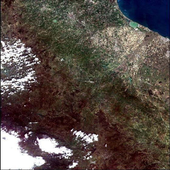
ATCOR Workflow for IMAGINE                         Step-by-Step Guide                             Page 10/33

7. Examine the Session Log.
8. Examine the project folder.

 Figure 8: Spatial model for processing the Landsat-8 data set (Example 1) using the ATCOR Workflow operators
 (1). The model creates a new ATCOR project (2), executes ATCOR Dehaze (3), sets parameters relevant for
 ATCOR-2 (4), and executes ATCOR-2 (5).

9. Open the original image and the dehazed image in the Viewer and compare (Figure 10).
    Original image: My_ATCOR_Workflow_Demo_Folder>\Example1\02_atcor_project_SM\
                    lc81990262013104lgn01.tif
    Dehazed image: \Example1\03_output_SM\
                  LC81990262013104LGN01_dh.tif
    Then load the haze map in the viewer and compare with the original / dehazed image.
    Haze map:        \Example1\03_output_SM\
                     LC81990262013104LGN01_haze_map.tif
    Use the Inquire Cursor to examine the pixel values of the haze map. You get the class IDs but not
    the names of the map categories (class names). To add the class names, continue with step 10.
10. Remove the haze map from the Viewer.
11. Navigate to the Spatial Modeler window ‘Operators’, open the group Attributes, and add the
    operator Raster Attribute Output by drag-and-drop to the Spatial Modeler Editor. Connect the
    operator with the Run ATCOR Dehaze operator as follows and as shown in Figure 9 (6):
              •   HazeMapFile → Filename
              •   HazeMapCategories → TableIn
12. Set the operator ports (via double-click) as follows:
              •   TableType: String
              •   Attribute:    Class_Names

© GEOSYSTEMS GmbH, 2020
ATCOR Workflow for IMAGINE Step-by-Step Guide Page 11/33
Figure 9: Spatial model for processing the Landsat-8 data set (Example 1). The model creates a new ATCOR
project (2), executes ATCOR Dehaze (3), sets parameters relevant for ATCOR-2 (4), executes ATCOR-2 (5),
and adds the class names of the haze map to its attribute table (6).
13. Again, save the Spatial Model to the file
\Example1\03_output_SM\
Create_dehaze_atcor2.gmdx
14. Right-click the Raster Attribute Output operator and select Run Just This.
15. Display the haze map: add the file to the viewer and use the Inquire Cursor to get the pixel
values. Now the class IDs are displayed.
16. Display the dehazed and atmospherically corrected image
\Example1\03_output_SM\
lc81990262013104lgn01_atcor2.tif
and the value-added products file
\Example1\03_output_SM\
lc81990262013104lgn01_atcor2_flx.tif.
By default, the file is located in the same directory as the atmospherically corrected image.
17. Display layer 2 (Leaf Area Index; Table 2) of the value-added products file (*_flx.tif) with File
– Open – Raster as Image Chain. Navigate to the Multispectral Tab, click the button Image
Chain (Group Settings), select Pseudocolor and select Layer 2 (Group View). Click the button
Color Table (Group Color) and select NDVI Natural.
Original Dehazed
Haze map Leaf area index (LAI)
© GEOSYSTEMS GmbH, 2020ATCOR Workflow for IMAGINE Step-by-Step Guide Page 12/33
Figure 10: Results of ATCOR Dehaze and ATCOR-2 for Example 1 (detail): original image (top left), dehazed and
atmospherically corrected image (top right), haze map (bottom left; yellowish colors indicate haze contaminated
pixels, see Table 1 for haze map categories), Leaf Area Index Index (LAI) (bottom right; brown: low LAI, green:
high LAI).
3 Example 2
3.1 What You Will Learn
Based on a Landsat-5 TM dataset (subset), the following processing steps are demonstrated:
• manual metadata input,
• calibration coefficients adjustment, and
• atmospheric and topographic correction in rugged terrain (ATCOR-3).
Note: For Landsat-5 TM data, ATCOR Workflow can import metadata information automatically from
the corresponding metadata file. For demonstration purposes, this example shows how metadata can
be entered manually. This is useful if the original metadata file is missing as well as for sensors without
automatic metadata import (e.g. GEOEYE-1).
The example data set is processed using the ATCOR Workflow Dialog (Section 3.3) and the ATCOR
Workflow Operators (Spatial Modeler) (Section 3.4).
3.2 Data Description
In this example we will use the subset of a Landsat-5 TM scene (Section 3.2.1) and the corresponding
SRTM subset (Section 3.2.2).
3.2.1 Landsat-5 TM Image
Quicklook:
(Band 5–4–3)
© GEOSYSTEMS GmbH, 2020ATCOR Workflow for IMAGINE Step-by-Step Guide Page 13/33
Sensor: Landsat-5 TM
Acknowledge- Landsat 5 TM image courtesy of the U.S. Geological Survey
ment:
Extent: Subset of scene 193/027 (path/row),
UL: X 616260.0 Y 5330130.0, LR: X 715290.0 Y 5256210.0,
UTM, Zone 32 (EPSG: 32632)
Band order: B10 - B20 - B30 - B40 - B50 - B60 - B70
Pixel size: 30 m (band B60 was resampled from 60 m to 30 m)
Data type: Unsigned 8-bit
Acquisition date: 2003-07-14
Sun azimuth: 132.91°
Sun elevation: 57.21°
Radiometric RADIANCE_ADD_BAND_1 = -2.28583 RADIANCE_MULT_BAND_1 = 0.7658
rescaling: RADIANCE_ADD_BAND_2 = -4.28819 RADIANCE_MULT_BAND_2 = 1.4482
[Wm-2sr-1µm-1]
RADIANCE_ADD_BAND_3 = -2.21398 RADIANCE_MULT_BAND_3 = 1.0440
RADIANCE_ADD_BAND_4 = -2.38602 RADIANCE_MULT_BAND_4 = 0.8760
RADIANCE_ADD_BAND_5 = -0.49035 RADIANCE_MULT_BAND_5 = 0.1204
RADIANCE_ADD_BAND_6 = 1.18243 RADIANCE_MULT_BAND_6 = 0.0554
RADIANCE_ADD_BAND_7 = -0. 21555 RADIANCE_MULT_BAND_7 = 0.0656
3.2.2 Digital Elevation Model
Mission: SRTM (Shuttle Radar Topography Mission)
Pixel size: 90 m
Acknowledge- USGS (2006), Shuttle Radar Topography Mission, 3 Arc Second scene, Global
ment: Land Cover Facility, University of Maryland, College Park, Maryland.
© GEOSYSTEMS GmbH, 2020ATCOR Workflow for IMAGINE Step-by-Step Guide Page 14/33
3.3 Data Processing Using the ATCOR Workflow Dialog
1. Download the file ATCOR_Workflow_Step_by_Step_Guide_Example2.zip
from http://www.geosystems.de/en/products/atcor-workflow-for-imagine/download
and extract it to the folder \Example2.
2. Create the following folders:
\Example2\02_atcor_project
\Example2\03_output
\Example2\04_elevation_repository_SM
3. Click Toolbox Tab > ATCOR Workflow for IMAGINE > Run ATCOR-3 to open the ATCOR-3
dialog.
4. Select the Operation Mode Create ATCOR Project.
5. Specify the following options on the Project Tab of the dialog:
• Project folder: navigate into the folder
\Example2\02_atcor_project
• Sensor: Landsat-4/5 TM
• Image File:
\Example2\01_data\Landsat5\
lt51930272003195mti01_subset.img
• Metadata File: [no input, as we do not have a metadata file]
• Elevation File:
\Example2\01_data\DEM\
dem_germany_90m_subset.img
• Corrected Image File: specify the name for the output file (new file)
\Example2\03_output\
lt51930272003195mti01_subset_atcor3.img
6. Navigate from the Project Tab to the Basic Settings Tab (Figure 11).
In the Sensor Information box and in the Geometry box default metadata values are shown.
They have to be modified according to the data description in Section 3.2:
• Pixel Size: 30
• Acquisition date: 2003-07-14
• Solar Zenith: 32.8 (= 90° - Sun Elevation)
• Solar Azimuth: 132.9
© GEOSYSTEMS GmbH, 2020ATCOR Workflow for IMAGINE Step-by-Step Guide Page 15/33
In the Atmosphere box specify the following parameters after checking the corresponding Edit
box:
• Water Vapor Category: mid-latitude summer
• Aerosol Type: rural
7. Navigate from the Basic Settings Tab to the Advanced Settings Tab (Figure 12) and edit the
following parameters:
Value-added Products Box:
• Compute Value-added Products: not checked
BRDF Correction Box:
• BRDF Model: (2b) specific, weak
• g: 0.200
• betaT: 0.0
We set betaT to 0.0 in order to get this parameter as a function of the solar zenith
angle. More details are provided in the User Manual
(ATCOR_Workflow_for_IMAGINE_Help.pdf).
Figure 11: Basic Settings Tab of ATCOR-3. Figure 12: Advanced Settings Tab of ATCOR-3.
Figure 13: DEM Settings Tab of ATCOR-3.
© GEOSYSTEMS GmbH, 2020ATCOR Workflow for IMAGINE Step-by-Step Guide Page 16/33
8. Navigate from the Advanced Settings Tab to the DEM Settings Tab (Figure 14).
The elevation repository (new since ATCOR Workflow for IMAGINE 2020) allows to store the
derivatives of the DEM to be stored permanently under a user-defined ID. If the same area is
processed later on using ATCOR 3, these files can be re-used, which saves a significant amount
of processing time.
Elevation and Derivatives Repository Box:
• Use Elevation Repository: checked.
• Elevation Repository Directory: \Example2\04_elevation_repository_SM
• Elevation Repository ID: landsat_001
• Replace Existing Repository: checked.
Scaling and DEM Processing Box:
• Reflectance Scale Factor: 4
• The output data type will be Unsigned 8-bit (same as input), i.e. values from 0 to 255
can be stored. Considering the expected range of surface reflectance values, a
reflectance scale factor of 4 would be suitable. With this scaling factor, a surface
reflectance of 20.56%, for example, is coded as 82.
• DEM Smoothing: -none-
9.
10. Click Run. Depending on your PC, processing will take about 5 minutes to finish. Check the
process status in the ERDAS IMAGINE Process List.
11. Examine the Session Log. Here you find some basic information about the executed process as
well as warnings or error messages if a problem occurred.
12. Examine the project folder:
\Example2\02_atcor_project
Here you find the following files:
• GEOSYSTEMS_ATCOR.project, the ATCOR project file, a text file containing some
basic information on the project,
• lt51930272003195mti01_subset_ele.tif, the elevation file prepared from
the specified elevation file to satisfy the ATCOR-specific requirements,
• lt51930272003195mti01_subset.log, the log file, and
• lt51930272003195mti01_subset.cal, the calibration file.
• Folder _Repository with some temporary results.
13. Examine the log file. Here you can find detailed information about the executed process.
14. Examine the Elevation Repository folder.
\Example2\04_elevation_repository_SM
Here you find the following files:
• asp_landsat_001.bsq / .hdr, the aspect file in .bsq format and the according header
file derived from the DEM
• ele_landsat_001.bsq /.hdr, the elevation file in .bsq format and the according header
file converted from the elevation file.
• sky_landsat_001.bsq /.hdr, the skyview file in .bsq format and the according header
file derived from the DEM
© GEOSYSTEMS GmbH, 2020ATCOR Workflow for IMAGINE Step-by-Step Guide Page 17/33
• slp_landsat_001.bsq /.hdr, the slope file in .bsq format and the according header file
derived from the DEM
For subsequent processing of this dataset, you can re-use these files by entering the same
ElevationRepositoryDirectory and RepositoryID again in order to save processing time.
15. Open the original image and the atmospherically/topographically corrected image in the Viewer
and compare (Figure 15), using for example the band composition 5 (Red) – 4 (Green) – 3 (Blue).
Original image: \Example2\01_data\Landsat5\
lt51930272003195mti01_subset.img
Corrected image: \Example2\03_output\
lt51930272003195mti01_subset_atcor3.img
16. Finally, we want to adjust the calibration parameters c0 (Offset) and c1 (Gain). Many sensors
are recalibrated from time to time. The actual calibration parameters are usually provided together
with the image or can be downloaded from the web. It is recommended to use the image-specific
parameters if available.
For the first run, we used default calibration parameters. So now let us replace them by the values
provided in Section 3.2 (Radiometric rescaling). For each spectral band, there are two values, i.e.
RADIANCE_ADD corresponding to the Offset and RADIANCE_MULT corresponding to the Gain.
It is important to pay attention to the unit. The values provided in Section 3.2 are based on the
radiance unit Wm-2sr-1µm-1, while ATCOR Workflow employs the unit mWcm-2sr-1µm-1. Thus, the
values have to be multiplied by the conversion factor 0.1, before they can be used in ATCOR
Workflow.
Open the calibration file
\Example2\02_atcor_project\
lt51930272003195mti01_subset.cal
in a text editor, edit the values as explained, and save them to a new text file:
\Example2\02_atcor_project\
lt51930272003195mti01_subset_V2.cal
The new calibration file will look like the text file shown in Figure 14. More information on the
calibration procedure is provided in the User Manual
(ATCOR_Workflow_for_IMAGINE_Help.pdf).
Figure 14: Calibration file according to the image-specific calibration parameters.
17. Click Toolbox Tab > ATCOR Workflow for IMAGINE > Run ATCOR-3 to open the ATCOR-3
dialog.
18. Select the Operation Mode Load ATCOR Project.
19. Specify the following options on the Project Tab of the dialog:
• Project folder: select the folder
\Example2\02_atcor_project
• Corrected Image File: specify the name for the output file (new file)
\Example2\03_output\
lt51930272003195mti01_subset_atcor3_V2.img
© GEOSYSTEMS GmbH, 2020ATCOR Workflow for IMAGINE Step-by-Step Guide Page 18/33
20. Navigate from the Project Tab to the Basic Settings Tab, check the Edit box of the calibration
file and select the new calibration file:
\Example2\02_atcor_project\
lt51930272003195mti01_subset_V2.cal
21. Navigate from the Basic Settings Tab to the Advanced Settings Tab. All settings are preserved
from the previous run. So you do not have to set them again.
22. Click Run. Depending on your PC, processing will take again a few minutes to finish. Check the
process status in the ERDAS IMAGINE Process List.
23. Display the result and compare the new output file with the first result. The new output file
appears slightly brighter than the first result. However, as the image-specific calibration
parameters (V2) are quite similar to the default parameters the difference is not significant.
Note: Adjusting the calibration parameters can also be useful, if the result of atmospheric
correction is not satisfying, e.g. if there are many pixels in the resulting image with a value of zero.
Figure 15: Comparison of the original (left) and the image corrected with ATCOR-3 (right) for the full
image (top) and a detail taken from the mountainous part in the south of the image (bottom). Band
composition 5-4-3.
© GEOSYSTEMS GmbH, 2020ATCOR Workflow for IMAGINE Step-by-Step Guide Page 19/33
3.4 Data Processing Using the ATCOR Workflow Operators
1. Download (if not done already following the instructions in Section 3.3) the file
ATCOR_Workflow_Step_by_Step_Guide_Example2.zip
from http://www.geosystems.de/en/products/atcor-workflow-for-imagine/download
and extract it to the folder \Example2\.
2. Create the following folders:
\Example2\02_atcor_project_SM
\Example2\03_output_SM
\Example2\04_elevation_repository_SM
3. Click Toolbox Tab > Spatial Model Editor to open the Spatial Modeler.
4. Navigate to the Operators window of the Spatial Modeler, open the group GEOSYSTEMS
ATCOR (Figure 16a, (1)), and add the operators Create ATCOR Project, Get ATCOR Elevation
Repository Options, Set ATCOR Parameters, and Run ATCOR-3 by drag-and-drop to the Spatial
Model Editor. Connect the operators as shown in Figure 16a.
5. Set the operator ports by double-clicking the ports as follows (see also Figure 16b):
Create ATCOR Project:
• ATCORProjectFolder: navigate into the folder
\Example2\02_atcor_project_SM
• ImageFilename:
\Example2\01_data\Landsat5\
lt51930272003195mti01_subset.img
• Sensor: Landsat-4/5 TM
• ElevationFilename:
\Example2\01_data\DEM\
srtm_germany_90m_subset.img
Get ATCOR Elevation Repository Options: To enable the ports, right-click the operator, select
Properties, and enable the ports RepositoryID, ElevationRepositoryDirectory and
ReplaceExisting in the Properties window located in the lower right corner of your screen. Again,
to set the ports, double-click the ports (not the operator) and select the following values:
• RepositoyID: landsat_001
© GEOSYSTEMS GmbH, 2020ATCOR Workflow for IMAGINE Step-by-Step Guide Page 20/33
• ElevationRepositoryDirectory: \Example2\04_elevation_repository_SM
• ReplaceExisting: true
Set ATCOR Parameters: To enable the ports, right-click the operator, select Properties, and
enable the ports in the Properties window located in the lower right corner of your screen. Again,
to set the ports, double-click the ports (not the operator) and select the following values according
to Section 3.2.1:
• PixelSize: 30
• AcquisitionDate: 2003-07-14
• SolarZenith: 32.8 (= 90°- Sun Elevation)
• SolarAzimuth: 132.9
• Water Vapor Category: mid-latitude summer
• Aerosol Type: rural
• ReflScaleFactor: 4
• BRDFModel: (2b) specific, weak
• BRDF-betaT: 0.0
• BRDF-g: 0.200
Additionally, enable the port “Options”, which later needs to be connected with the output port of
the Get ATCOR Elevation Repository Options operator (Figure 16: Spatial model for processing
the Landsat-5 data set (Example 2). The model involves four operators from the group
GEOSYSTEMS ATCOR (1). It creates a new ATCOR project (2), sets options for the elevation
repository (3), sets metadata and processing parameters (4), and executes ATCOR-3 (5).
Figure (a) shows the operators before setting the ports, in Figure (b) the ports are set as required
to process the dataset..
The output data type will be Unsigned 8-bit (same as input), i.e. values from 0 to 255 can be
stored. Considering the expected range of surface reflectance values, a reflectance scale factor
of 4 would be suitable. With this scaling factor, a surface reflectance of 20.56%, for example, is
coded as 82.
We set BRDF-betaT to 0.0 in order to get this parameter as a function of the solar zenith angle.
The applied rules are given in the User Manual (ATCOR_Workflow_for_IMAGINE_Help.pdf).
Run ATCOR-3:
• CorrectedImageName: specify the name of the output file (new file)
\Example2\03_output_SM\
lt51930272003195mti01_subset_atcor3.img
6. Save the Spatial Model, for example to the file
\Example2\03_output_SM\
Create_atcor3.gmdx
7. Click Run in the Spatial Modeler Tab. Depending on your PC, the processing will take about 5
minutes to finish. Check the process status in the ERDAS IMAGINE Process List.
8. Examine the Session Log.
9. Examine the project folder.
\Example2\02_atcor_project_SM
© GEOSYSTEMS GmbH, 2020ATCOR Workflow for IMAGINE Step-by-Step Guide Page 21/33
Here you find the following files:
• GEOSYSTEMS_ATCOR.project, the ATCOR project file, a text file containing some
basic information on the project,
• lt51930272003195mti01_subset_ele.tif, the elevation file prepared from
the specified elevation file to satisfy the ATCOR-specific requirements,
• lt51930272003195mti01_subset.log, the log file, and
• lt51930272003195mti01_subset.cal, the calibration file.
10. Examine the Elevation Repository folder.
\Example2\04_elevation_repository_SM
Here you find the following files:
• asp_landsat_001.bsq
• asp_landsat_001.hdr
• ele_landsat_001.bsq
• ele_landsat_001.hdr
• sky_landsat_001.bsq
• sky_landsat_001.hdr
• slp_landsat_001.bsq
• slp_landsat_001.hdr
These files are aspect, slope, skyview and elevation files as required by ATCOR3.
For subsequent processing of this dataset, you can re-use these files by entering the same
ElevationRepositoryDirectory and RepositoryID again in order to save processing time.
11. Open the original image and the corrected image in the Viewer and compare (Figure 15).
Original image: \Example2\01_data\Landsat5\
lt51930272003195mti01_subset.img
Corrected image: \Example2\03_output_SM\
lt51930272003195mti01_subset_atcor3.img
© GEOSYSTEMS GmbH, 2020ATCOR Workflow for IMAGINE Step-by-Step Guide Page 22/33
(a)
(b)
Figure 16: Spatial model for processing the Landsat-5 data set (Example 2). The model involves four operators
from the group GEOSYSTEMS ATCOR (1). It creates a new ATCOR project (2), sets options for the elevation
repository (3), sets metadata and processing parameters (4), and executes ATCOR-3 (5). Figure (a) shows the
operators before setting the ports, in Figure (b) the ports are set as required to process the dataset.
12. Finally, we want to adjust the calibration parameters c0 (Offset) and c1 (Gain). Many sensors
are recalibrated from time to time. The actual calibration parameters are usually provided together
with the image or can be downloaded from the web. It is recommended to use the image-specific
parameters if available.
For the first run, we used default calibration parameters. So now let us replace them by the values
provided in Section 3.2 (Radiometric rescaling). For each spectral band, there are two values, i.e.
RADIANCE_ADD corresponding to the Offset and RADIANCE_MULT corresponding to the Gain.
It is important to pay attention to the unit. The values provided in Section 3.2 are based on the
radiance unit Wm-2sr-1µm-1, while ATCOR Workflow employs the unit mWcm-2sr-1µm-1. Thus, the
values have to be multiplied by the conversion factor 0.1, before they can be used in ATCOR
Workflow.
Open the calibration file
\Example2\02_atcor_project_SM\
lt51930272003195mti01_subset.cal
in a text editor, edit the values as explained, and save them to a new text file:
\Example2\02_atcor_project_SM\
lt51930272003195mti01_subset_V2.cal
The new calibration file will look like the text file shown in Figure 17. More information on the
calibration issue is provided in the User Manual (ATCOR_Workflow_for_IMAGINE_Help.pdf).
© GEOSYSTEMS GmbH, 2020ATCOR Workflow for IMAGINE Step-by-Step Guide Page 23/33
Figure 17: Calibration file according to the image-specific calibration parameters.
13. Enable the port ‘CalibrationFilename’ of the ‘Set ATCOR Parameters’ operator and select the
new calibration file
\Example2\02_atcor_project_SM\
lt51930272003195mti01_subset_V2.cal
Alternatively, you can double-click the ‘Set ATCOR Parameters’ operator. A dialog opens. Select
the Standard Tab. In the box ‘File and Sensor Information’ you can select the new calibration file.
14. Modify the output file name specified at the port ‘CorrectedImageName’ of the operator ‘Run
ATCOR-3’ to avoid that the previous output file is replaced:
\Example2\03_output_SM\
lt51930272003195mti01_subset_atcor3_V2.img
15. Click Run in the Spatial Modeler Tab. As now only the processes ‘Set ATCOR Parameters’ and
‘Run ATCOR-3’ are executed, the processing will be much faster than the first time you executed
the model.
16. Display the result and compare the new output file with the first result. The new output file
appears slightly brighter than the first result. However, as the image-specific calibration
parameters (V2) are quite similar to the default parameters, the difference is not significant in this
example.
Note: Adjusting the calibration parameters can also be useful, if the result of atmospheric
correction is not satisfying, e.g. if there are many pixels in the resulting image with a value of zero.
© GEOSYSTEMS GmbH, 2020ATCOR Workflow for IMAGINE Step-by-Step Guide Page 24/33
4 Example 3
4.1 What you Will learn
Based on a Sentinel-2 image, the following processing steps are demonstrated:
• Automatic metadata import,
• Haze reduction (ATCOR Dehaze), and
• Atmospheric correction in flat terrain (ATCOR-2)
The example data set (Figure 18 and Figure 19) is processed using the ATCOR Workflow Dialog
(Section 4.2) and the ATCOR Workflow Operators (Spatial Modeler) (Section 4.3).
Figure 18: Footprint of the Sentinel-2 demo data set Figure 19: True color quicklook of the Sentinel-2
(Example 3), Product URI: demo data set.
S2A_MSIL1C_20170319T095021_N0204_R079_
T33TWF_20170319T095021.SAFE.
4.2 Data processing Using the ATCOR Workflow Dialog
Run ATCOR Dehaze:
From the Toolbox menu in IMAGINE 2020 open the ATCOR Workflow for IMAGINE menu and start
Run ATCOR Dehaze.
1. Create the following folders:
\Example3\02_atcor_project
\Example3\03_output
In Tab Project choose Create ATCOR Project insert the following:
• Input:
o Project Folder:
\Example3\02_atcor_project
© GEOSYSTEMS GmbH, 2020ATCOR Workflow for IMAGINE Step-by-Step Guide Page 25/33
o Sensor: Sentinel-2 13 bands
o Image File (do not use the manifest.safe file!):
\Example3\01_S2_data\
S2A_MSIL1C_20170319T095021_N0204_R079_T33TWF_20170319T095021.SAFE\
GRANULE\L1C_T33TWF_A009085_20170319T095021\MTD_TL.xml
• Output:
o Dehazed Image:
\Example3\03_output\
Sentinel2_13Bands_Napoli_dh.tif
In Tab Settings set:
• Dehazing Parameters:
o DehazeMethod: standard
o DehazeArea: land and water pixels
o DehazedImageName:
\Example3\03_output\
Sentinel2_13Bands_Napoli_dh.tif
o Check Use Cirrus Band If Available
o Interpolation Method: bilinear (fast)
© GEOSYSTEMS GmbH, 2020ATCOR Workflow for IMAGINE Step-by-Step Guide Page 26/33
Then click the Run button.
Run ATCOR 2:
From the Toolbox menu in IMAGINE 2020 open the ATCOR Workflow for IMAGINE menu and start
Run ATCOR 2.
In Tab Project choose Load ATCOR Project insert the following:
• Project Folder: \Example3\02_atcor_project
• Corrected Image: \Example3\03_output\
Sentinel2_13Bands_Napoli_dh_atcor2.tif
In Tab Advanced Settings check boxes Edit in the AOT File group and in the Water Vapor File group
and insert:
• AOT File: \Example3\03_output\
Sentinel2_13Bands_Napoli_dh_atcor2_aot.tif
© GEOSYSTEMS GmbH, 2020ATCOR Workflow for IMAGINE Step-by-Step Guide Page 27/33
• Water Vapor File: \Example3\03_output\
Sentinel2_13Bands_Napoli_dh_atcor2_wv.tif
• Cloud Shadow Water File: \Example3\03_output\
Sentinel2_13Bands_Napoli_dh_atcor2_csw.tif
Click Run and examine the results according to 4.3 (see below).
4.3 Data processing Using the ATCOR Workflow Operators
2. Create the following folders:
\Example3\02_atcor_project_SM
\Example3\03_output_SM
3. Click Toolbox Tab > Spatial Model Editor to open the Spatial Modeler.
4. Navigate to the Operators window, open the group GEOSYSTEMS ATCOR, and add the
operators Create ATCOR Project, Run ATCOR Dehaze, Set ATCOR Parameters, and Run
ATCOR-2 by drag-and-drop to the Spatial Model Editor. Connect the operators as shown in
Figure 20.
5. Set the operator ports as follows (see also Figure 20) by double-clicking the corresponding ports:
Create ATCOR Project:
• ATCORProjectFolder: navigate into the folder
\Example3\02_atcor_project_SM
• ImageFilename: switch off the file filter ‘All File-based Raster Formats’ by entering
‘*.xml’ in the field ‘Image File’ and select the file
\Example3\01_S2_data\
S2A_MSIL1C_20170319T095021_N0204_R079_T33TWF_20170319T095021.SAFE
\
GRANULE\L1C_T33TWF_A009085_20170319T095021\MTD_TL.xml
• Sensor: Sentinel-2 13 Bands
© GEOSYSTEMS GmbH, 2020ATCOR Workflow for IMAGINE Step-by-Step Guide Page 28/33
Run ATCOR Dehaze:
• DehazeMethod: standard
• DehazeArea: land and water pixels
• DehazedImageName:
\Example3\03_output_SM\
Sentinel2_13Bands_Napoli_dh.tif
Set ATCOR Parameters: Enable the ports by right-clicking the operator, select Properties. The
Properties window is now located in the lower right corner of your screen. Enable the ports by
checking the port in the ‘Show’ column. To set the port, double-click the port (not the operator) and
select the following values:
• Water Vapor Category: fall/spring
• Aerosol Type: rural
• ValueAddedProds: true
The computation of the value-added products file can also be enabled (not
recommended here!) by using the ‘Set ATCOR Parameters’ GUI. It is opened by
double-clicking the operator. The processing parameter Compute Value-added
Products is located on the Advanced Settings Tab of the GUI. Before the GUI
opens, the Create ATCOR Project operator is executed. Thus, it is recommended to
enter the parameters via the ports and not via the GUI, when the project has not
been created yet. However, you might find the GUI useful in combination with the
‘Load ATCOR Project’ operator.
Run ATCOR-2:
• CorrectedImageName:
\Example3\03_output_SM\
Sentinel2_13Bands_Napoli_dh_atcor2.tif
The atmospheric correction (ATCOR-2) is executed on the dehazed image.
• AOTFilename: \Example3\03_output\Sentinel2_13Bands_Napoli_dh_atcor2_
aot.tif
• WaterVaporFileName: \Example3\03_output\Sentinel2_13Bands_Napoli_dh_atcor2_
wv.tif
• CloudShadowWaterFile: \Example3\03_output\Sentinel2_13Bands_Napoli_dh_atcor2_
csw.tif
6. Save the Spatial Model, for example to the file
\Example3\03_output_SM\
Create_dehaze_atcor2.gmdx
7. Click Run in the Spatial Modeler Tab. Depending on your PC, the processing will take about 10
minutes to finish. Check the process status in the ERDAS IMAGINE Process List.
When the process finished successfully, you can see a warning icon at the ‘Run ATCOR Dehaze’
operator and an info icon at the ‘Run ATCOR-2’ operator. See the Spatial Modeler Messages window
for more information. You can open this window by clicking the ‘Messages’ button in the Spatial
Modeler ribbon (group ‘View’).
8. Examine the Session Log.
9. Examine the project folder.
© GEOSYSTEMS GmbH, 2020ATCOR Workflow for IMAGINE Step-by-Step Guide Page 29/33
Figure 20: Spatial model for processing the Sentinel-2 data set (Example 3) using the ATCOR Workflow operators
(1). The model creates a new ATCOR project (2), executes ATCOR Dehaze (3), sets parameters relevant for
ATCOR-2 (4), and executes ATCOR-2 (5).
10. Open the original image and the dehazed image in the Viewer and compare (Figure 22). Use a
proper LUT stretch function to improve the contrast of the image.
Original image: My_ATCOR_Workflow_Demo_Folder>\Example3\02_atcor_project_SM\
TOA_reflectance\S2A_OPER_MSI_L1C_TL_SGS__20170319T133044_A00
9085_T33TWF_N02_04.tif
Dehazed image: \Example1\03_output_SM\
Sentinel2_13Bands_Napoli_dh.tif
Now load the haze map into the viewer and compare with the original / dehazed image.
Haze map: \Example3\03_output_SM\
Sentinel2_13Bands_Napoli_haze_map.tif
Use the Inquire Cursor to examine the pixel values of the haze map. You get the class IDs but not
the names of the map categories (class names). To add the class names, continue with step 10.
11. Remove the haze map from the Viewer.
12. Navigate to the Spatial Modeler window ‘Operators’, open the group Attributes, and add the
operator Raster Attribute Output by drag-and-drop to the Spatial Modeler Editor. Connect the
operator with the Run ATCOR Dehaze operator as follows and as shown in Figure 9 (6):
• HazeMapFile → Filename
• HazeMapCategories → TableIn
13. Set the operator ports (via double-click) as follows:
• TableType: String
• Attribute: Class_Names
© GEOSYSTEMS GmbH, 2020ATCOR Workflow for IMAGINE Step-by-Step Guide Page 30/33
Figure 21: Spatial model for processing the Sentinel-2 data set (Example 3). The model creates a new ATCOR
project (2), executes ATCOR Dehaze (3), sets parameters relevant for ATCOR-2 (4), executes ATCOR-2 (5),
and adds the class names of the haze map to the its attribute table (6).
14. Again, save the Spatial Model to the file
\Example3\03_output_SM\
Create_dehaze_atcor2.gmdx
15. Right-click the Raster Attribute Output operator and select Run Just This.
16. Display the haze map: add the file to the viewer and use the Inquire Cursor to get the pixel
values. Now the class names are displayed together with the class IDs.
17. Display the dehazed and atmospherically corrected image
\Example3\03_output_SM\
Sentinel2_13Bands_Napoli_dh_atcor2.tif
and the value-added products file
\Example3\03_output_SM\
Sentinel2_13Bands_Napoli_dh_atcor2_flx.tif.
By default, the value-added products file is located in the same directory as the atmospherically
corrected image.
18. Display layer 1 (Soil-adjusted Vegetation Index; Table 2) of the value-added products file
(*_flx.tif) with File – Open – Raster as Image Chain. Navigate to the Multispectral Tab, click
the button Image Chain (Group Settings), select Pseudocolor and select Layer 1 (Group View).
Click the button Color Table (Group Color) and select NDVI Natural.
19. Display the aerosol optical thickness file \Example3\03_output\Sentinel2_13Bands_Napoli_dh_atcor2_aot.tif
and inspect the values using the Inquire tool.
20. Display the water vapor file \Example3\03_output\ Sentinel2_13Bands_Napoli_dh_atcor2_wv.tif
and inspect the values using the Inquire tool.
21. Display the Cloud-Shadow-Water Map (CSW-Map) \Example3\03_output\
Sentinel2_13Bands_Napoli_dh_atcor2_out_csw.tif and compare it visually to the
Haze Map. The class names of the CSW-Map can be attached to the raster similar as for the Haze
Map, described above (Figure 21).
© GEOSYSTEMS GmbH, 2020ATCOR Workflow for IMAGINE Step-by-Step Guide Page 31/33 Original Dehazed Haze map Soil-adjusted vegetation index (SAVI) Figure 22: Results of ATCOR Dehaze and ATCOR-2 for Example 3 (detail): original image (top left), dehazed and atmospherically corrected image (top right), haze map (bottom left; yellowish colors indicate haze contaminated pixels, see Table 1 for haze map categories), Leaf Area Index Index (LAI) (bottom right; brown: low LAI, green: high LAI). © GEOSYSTEMS GmbH, 2020
ATCOR Workflow for IMAGINE                         Step-by-Step Guide                            Page 32/33

5 Appendix

Table 1: Haze map categories.

   Color     Class ID    Class Name                   Comment

                 0       geocoded background          --

                 1       shadow                       --

                 2       thin cirrus (water)          --

                 3       medium cirrus (water)        --

                 4       thick cirrus (water)         --

                 5       land (clear)                 --

                 6       saturated                    --

                 7       snow/ice (ice cloud)         --

                 8       thin cirrus (land)           --

                 9       medium cirrus (land)         --

                10       thick cirrus (land)          --

                11       haze (land)                  --

                12       medium haze (land)           --

                13       haze (water)                 --

                14       med. haze/glint (water)      --

                15       cloud (land)                 Haze removal limited due to physical reasons.

                16       cloud (water)                Haze removal limited due to physical reasons.

                17       water                        --

                18       cirrus cloud                 Haze removal maybe limited due to physical reasons.

                19       cirrus cloud (thick)         Haze removal limited due to physical reasons.

                20       bright                       --

                21       topographic shadow           --

© GEOSYSTEMS GmbH, 2020
ATCOR Workflow for IMAGINE Step-by-Step Guide Page 33/33
Table 2: Layers of the value-added products file.
Layer Name
1 Soil-adjusted vegetation index (SAVI), range 0 to 1000, scaled with factor 1000.
(e.g. scaled SAVI=500 corresponds to SAVI=0.5)
2 Leaf area index (LAI), range 0 to 10000, scaled with factor 1000.
(e.g. scaled LAI=5000 corresponds to LAI=5.0)
3 Fraction of photosynthetically active radiation FPAR, range 0 to 1000, scaled with factor 1000.
(e.g. scaled FPAR=500 corresponds to FPAR=0.5)
4 Surface albedo (integrated reflectance from 0.3 to 2.5 µm), range 0 to 1000, scaled with factor 10.
(e.g. scaled albedo=500 corresponds to albedo=50%)
5 Absorbed solar radiation flux Rsolar [W m-2].
6 Global radiation Eg [W m-2].
(omitted for constant visibility in flat terrain because it is a scalar that is written to the log file (*.log))
7 Thermal air-surface-flux-difference Rtherm = Ratm – Rsurface [W m-2].
8 Ground heat flux G [W m-2].
9 Sensible heat flux H [W m-2].
10 Latent heat LE [W m-2].
11 Net radiation Rn [W m-2].
© GEOSYSTEMS GmbH, 2020You can also read