Understanding gravity gradients a tutorial - AFIF H. SAAD, THE LEADING EDGE AUGUST 2006
←
→
Page content transcription
If your browser does not render page correctly, please read the page content below
Understanding gravity gradients
         ― a tutorial

           AFIF H. SAAD,
  Saad GeoConsulting, Richmond, Texas, USA

           THE METER READER

        THE LEADING EDGE
          AUGUST 2006
THE METER READER
      Coordinated by Bob Van Nieuwenhuise

      Understanding gravity gradients—a tutorial
      AFIF H. SAAD, Saad GeoConsulting, Richmond, Texas, USA

  T  he use of gravity gradient (GG) data in exploration is
  becoming more common. However, interpretation of grav-
  ity gradient data is not as easy as the familiar vertical grav-
  ity data. For a given source, regardless of its simplicity,
  gravity gradients often produce a complex pattern of anom-
  alies (single, doublet, triplet, or quadruplet) as compared
  to the simple single (monopolar) gravity anomalies. This
  paper is a minitutorial on gravity gradients and is designed
  to provide a simple explanation of the complex pattern of
  GG anomalies and suggest some guidelines for the inter-
  pretation of measured surface GG data.
      To demonstrate the complex pattern of anomalies asso-
  ciated with gravity gradients, I will compute the gravity gra-
  dient components of the full gradient tensor starting with
  the basic building block, the gravitational potential. This will
  be followed by computing and examining:

  • the first derivatives of the potential in x, y, and z direc-
    tions (i.e., the horizontal and vertical components of the
    gravity field vector)
  • the second derivatives of the potential (x-, y-, and z-
    derivatives of each gravity vector component) which
    constitute the nine components of the full GG tensor (of
    which only five are independent).

      Figure 1 shows the model, constructed with GOCAD,
  used for these computations—a diapiric salt body in a sed-          Figure 1. GOCAD salt model and Cartesian coordinates system used.
  imentary section whose density increases with depth, in a
  geologic setting typical of the U.S. Gulf coast. The upper part
  of the salt is above the “nil” zone and, thus, has positive den-
  sity contrasts with the surrounding sediments; the lower
  part of the salt body has negative density contrasts. The nil
  zone, at depth of about 1 km in this example, is the area where
  the density of the surrounding sediments is identical to that
  of salt; hence, its gravity effect is nil (Figure 2).
      This model is very realistic and useful because it was
  digitized from a real case history and is really two models
  in one—a shallow one with positive density contrasts, and
  a deeper one with negative density contrasts. Hence, it is
  useful for testing the resolving capabilities of gravity gra-
  dients from shallow to deep sources.

  The gravitational potential and its first derivatives. Figure
  3 shows color contour maps of the gravitational potential
  (P) and its first derivatives in the x, y, and z directions (P,x;
  P,y; and P,z). These derivatives are the horizontal (P,x; P,y)
  and vertical (P,z) gravity components of the gravity field vec-     Figure 2. Density-depth curves for salt and sediments typical of
  tor. The salt model depth contours (0.2, 0.5, 1, 2, 3, 4, 5, and    Gulf of Mexico geologic setting.
  6 km) are projected on all the maps for reference and to aid
  in interpretation.                                                  tion that produces the enhanced details and complex anom-
       The potential (P) shows mainly a broad bell-shaped neg-        alies of the gravity and gravity gradient components shown
  ative anomaly due to the main salt body; the effect of the          later.
  shallow part of the salt is not obvious although, on closer             The first horizontal derivatives of the potential in x and
  examination, there is a subtle change in the contour spac-          y or E and N directions produce doublet anomalies, a neg-
  ing in the northeast, suggesting a small positive anomaly.          ative–positive pair along the x and y axes, respectively
  It is interesting to note that, in spite of the apparent sim-       (Figure 3, top row). These are equivalent to the horizontal
  plicity of the potential anomaly, it contains all the informa-      gravity components gx and gy that would be measured by

942    THE LEADING EDGE   AUGUST 2006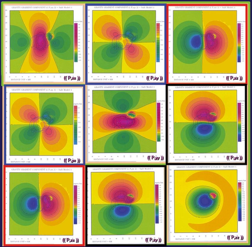
Figure 3. Gravitational potential P and its first derivatives P,x, P,y, and P,z (x-, y-, and z-gravity field components of the gravity vector g due to the
salt model shown).

                                                                                Figure 5. Frequency responses and characteristics of first derivative fil-
                                                                                ters: horizontal derivatives (left), vertical derivative (right).

                                                                                 should expect this pattern of gravity anomalies if we con-
                                                                                 sider the characteristic properties of the horizontal deriva-
                                                                                 tives. The horizontal derivative operator is a phase filter (left
                                                                                 panel in Figure 5) which will shift the location of anomalies
Figure 4. First horizontal derivative of P in the NE direction.                  or, in this case, split the negative P anomaly into a negative-
                                                                                 positive pair along the x- or y-axis, respectively. The fre-
a horizontal gravimeter. The pattern of doublet anomalies                        quency response of Ꭿ/Ꭿx, for example, is ikx where i is the
is coordinate-dependent as suggested by the rotated pattern                      imaginary number, and kx is the wavenumber in the x direc-
in Figure 4 for the NE directional horizontal derivative. We                     tion. Hence, the x-derivative involves a phase transforma-
                                                                                                                      AUGUST 2006      THE LEADING EDGE      943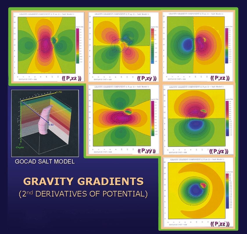
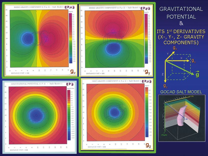
Figure 6. Gravity gradients (second derivatives of the potential).

  tion as well as enhancement of high fre-                                                        the potential P (Figure 3) has a negative
  quencies (or high wavenumbers) relative                                                         slope on the west and south sides of the
  to low frequencies. The phase transfor-                                                         minimum (going “downhill”), zero slope
  mation generally produces anomaly                                                               at the minimum, and positive slope on
  peaks (or troughs) approximately over                                                           the east and north sides (going
  the source edges in the case of wide bod-                                                       “uphill”)—thus producing the negative-
  ies (width w is large relative to depth d,                                                      positive pairs of gravity anomalies P,x
  w > d). The enhancement of high                                                                 and P,y. Notice that we can obtain the P,y
  wavenumbers sharpens these peaks to                                                             pattern of anomalies by a simple 90°
  increase the definition of body edges in                                                        counterclockwise rotation of the P,x pat-
  addition to emphasizing the effects of                                                          tern, in the same manner as one rotates
  shallow sources. Another explanation,                                                           the x-axis to the y-axis. In fact, if we rotate
  from elementary calculus, is that in the                                                        the x- and y- axes 45° counterclockwise,
  space domain the horizontal derivative                                                          or if we take the directional horizontal
  is defined as the rate of change of P with                                                      derivative of the potential P in the NE
  respect to x or y. Hence, the horizontal                                                        direction, the negative-positive pattern
  derivative is a measure of the slope or                                                         of anomalies obtained is rotated in the
  “gradient” of the anomalies in the x or                                                         same direction as shown in Figure 4,
  y direction (Figure 5, bottom left). If we            Figure 7. Frequency responses of second   emphasizing the fact that these anom-
  consider the P surface as topography,                 derivative filters.                       alies are coordinate-dependent.

944   THE LEADING EDGE    AUGUST 2006
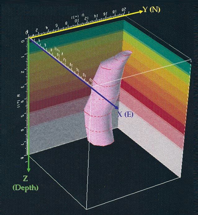
Figure 8. The full gravity gradient tensor.

     The first vertical derivative, on the other hand, is a zero-   response to the positive density contrast of the salt as com-
phase filter (right panel of Figure 5); hence, it will not affect   pared to the deeper salt effect.
the location of anomaly peaks, but it will sharpen the poten-
tial anomalies and will emphasize the high-frequency com-           The second derivatives of the potential. The various grav-
ponents due to shallow sources relative to the deeper effects,      ity gradient components are computed by taking the hori-
as seen in the P,z map of Figure 3 (lower right). The vertical      zontal x- and y-derivatives and vertical z-derivative of each
derivative of P is, by definition, the rate of change of P with     of the three gravity components of Figure 3. Figure 6 shows
depth; hence, its effect will be similar to downward continu-       the five independent components of the gravity gradient ten-
ation, making the anomalies sharper and emphasizing shal-           sor (second derivatives of the potential P): P,xx; P,xy; P,xz;
lower effects. Notice that the P,z data are the vertical gravity    P,yy; and P,yz along with the dependent second vertical
component gz measured by modern-day gravimeters.                    derivative P,zz (P,zz = –P,xx –P,yy by Laplace’s equation).
     The frequency response of all three first derivative fil-      Again, we can expect the single, double, triple, and quadru-
ters (Figure 5) is proportional to the wavenumber; hence,           ple pattern of anomalies produced, if we keep in mind the
we expect these derivatives to enhance the short wave-              properties and effect of the derivative operators explained
lengths or high frequencies due to the shallow part of the          above, or the frequency responses of the second derivative
salt with positive density contrast as suggested by the bend-       filters shown in Figure 7.
ing or embayment of the contours at that location in Figure              The gravity gradient component P,xx is computed by tak-
3. Notice the reverse polarity of the shallow anomalies in          ing the x-derivative of P,x. This results in a second phase
                                                                                                  AUGUST 2006   THE LEADING EDGE   945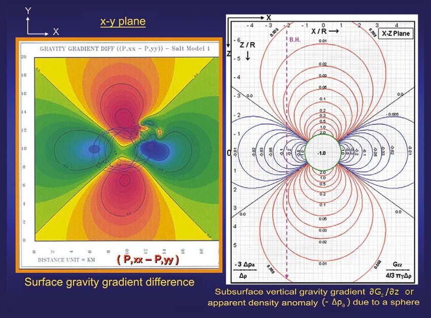
Figure 9. Combined products of gravity gradient components: Horizontal gradient and total gradient of gz.

                                                                                                              Figure 10. Combined
                                                                                                              products of gravity gradi-
                                                                                                              ent components:
                                                                                                              Differential curvature
                                                                                                              magnitude.

946   THE LEADING EDGE   AUGUST 2006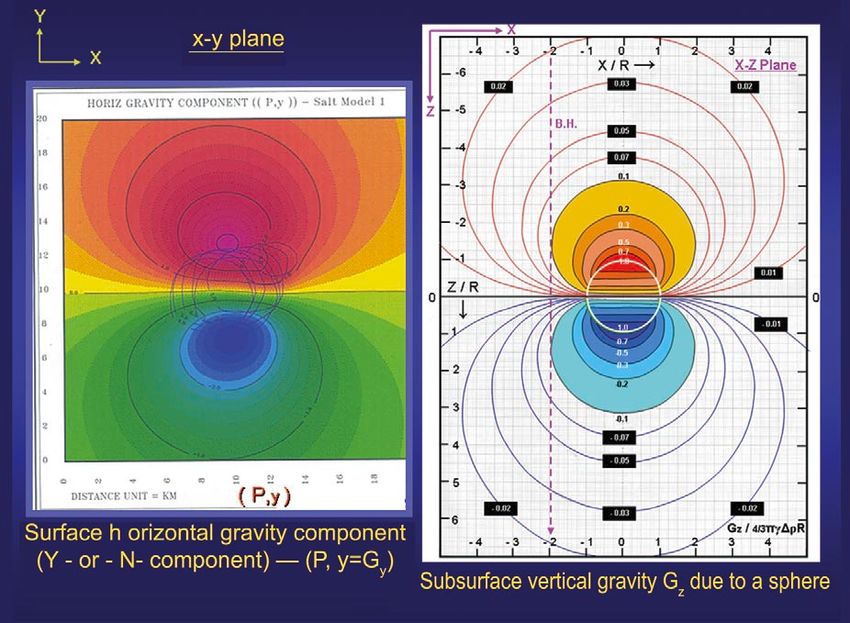
Figure 11. Gravity gradient invariants (after Pedersen and Rasmussen,   Figure 12. Other gravity gradient combinations: Euler deconvolution
1990).                                                                  using GG tensor components.

transformation and further enhancement of the high fre-                 tion. Thus, the tensor has only five independent components.
quencies of the anomalies of P,x. Thus, the negative anom-              It is interesting to note from Figure 8 that the first (top) row
aly of the doublet of P,x splits into a negative-positive pair,         of the tensor is identical with the first (left) column and its
and the positive anomaly splits into a positive-negative pair           components are the x-, y- and z-derivatives of the gravity
west-to-east along the x-axis, resulting into a “negative-              field horizontal component gx of the gravity vector g (Figure
strong positive–negative” triplet (P,xx of Figure 6). We can            3). Similarly, the second (center) row of the tensor is iden-
also explain this pattern by examining the slopes of the                tical with the second (center) column and its components
anomalies of P,x as we proceed from left to right along the             are the x-, y- and z-derivatives of the horizontal gravity field
x-axis. Notice that the steepest slope is at the center of the          component gy of the gravity vector g; the third (bottom) row
map of P,x (Figure 3) and it is positive; the zero slopes are           of the tensor is identical with the third (right) column and
at the trough and peak of P,x, and the gentle negative slopes           its components are the x-, y- and z-derivatives of the grav-
are to the left and right of the trough and peak, respectively.         ity field vertical component gz of the gravity vector g.
In a similar manner, we can explain the triplet pattern of                   Notice the greater enhancement and better definition of
the component P,yy (center panel of Figure 6) which is sim-             the shallow anomaly pattern associated with the upper part
ply a 90° counterclockwise rotation of the P,xx pattern.                of the salt in all gravity gradient maps (Figure 6). This is
    The gravity gradient component P,xy is computed by tak-             because the frequency response of all second derivative fil-
ing the derivative of P,x in the y (or N) direction or by tak-          ters is proportional to the square of the wave number (Figure
ing the derivative of P,y in the x (or E) direction. This results       7). Notice also the reverse polarity of the high-frequency
in a second phase transformation and further enhancement                anomaly pattern in all components as expected from the pos-
of high-frequencies of the anomalies of P,x or P,y.                     itive density contrast of the shallow salt. Thus, for example,
Considering P,x, the negative anomaly of the doublet of P,x             the triplet of P,xx is “positive-negative-positive” for shallow
splits into a negative-positive pair, along the y-direction or          salt as compared to the main “negative-positive-negative”
south-to-north and the positive anomaly splits into a posi-             pattern for the deep salt.
tive-negative pair along the y-direction or south-to-north,                  One should emphasize that the pattern of anomalies
resulting in a “negative-positive–negative–positive”                    produced is coordinate-dependent. However, one can use
quadruplet (P,xy of Figure 6, top center panel). We can also            these patterns and shapes of gravity gradient anomalies
explain this pattern by examining the slopes of the anom-               with the projected outline of the causative salt body in this
alies of P,x in Figure 3 as we proceed from south-to-north              example to develop interpretation techniques for locating
in the y-direction, or the slopes of the anomalies of P,y as            the main salt body, its edges, and its shallow part. For exam-
we proceed from west-to-east in the x-direction.                        ple, the zero contours of P,xx and P,yy closely define the west-
    The gravity gradient components P,xz and P,yz and P,zz              east edges and south-north edges of the main salt body,
(right column of Figure 6) are com-
puted by taking the z-derivative of P,x
and P,y and P,z, respectively. This only
causes further sharpening of the anom-
alies and enhancements of the high fre-
quencies of P,x and P,y and P,z without
any changes in the location or shapes
of the anomalies, the z-derivative being
a zero-phase filter (Figure 7).
    The full gradient tensor can be con-
structed by noting that P,yx = P,xy and
P,zy = P,yz and P,zx = P,xz (Figure 8).
The tensor is symmetric about its diag-
onal and its trace, the sum of the diag-
onal components (P,xx + P,yy + P,zz), is
identically equal to zero in source-free
regions, according to Laplace’s equa-

                                                                                                          AUGUST 2006     THE LEADING EDGE    947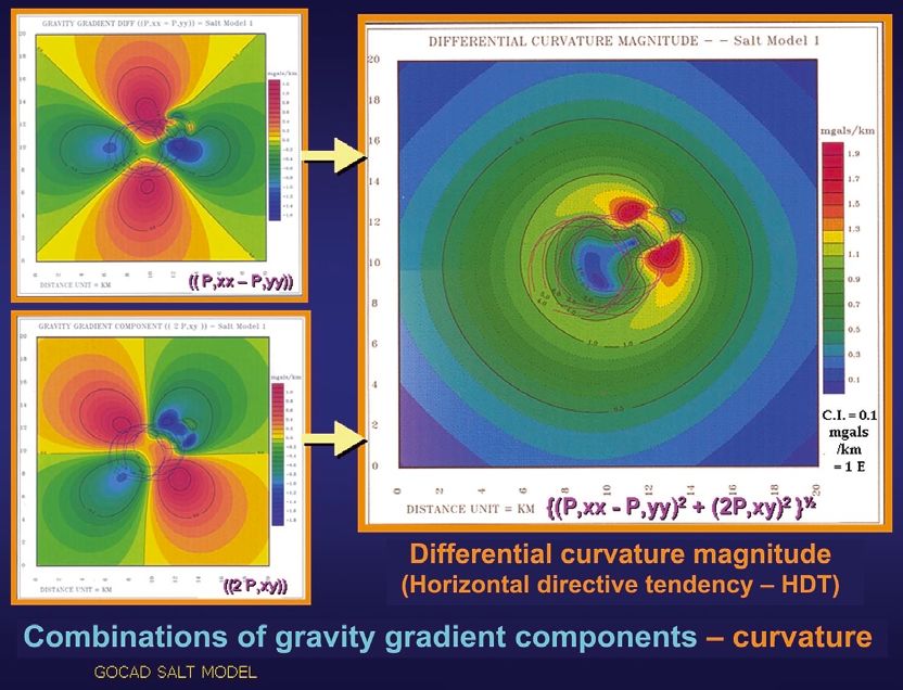
tions discussed above do not hold in
this case; the locations of the zero con-
tours, the lows and highs, and size of
the anomalies in general will depend
mainly on the depth to the source,
rather than the width/depth ratio.
Finally, the P,zz anomalies (Figure 6,
bottom-right panel) can be used to
locate the center of the anomalous
source mass.
Combinations of GG components
(invariants). Various combinations of
the gravity gradient components can
be used to simplify their complex pat-
tern and to further enhance and aid in
the interpretation of the data. Figures
9 and 10 show three examples: ampli-
tude of the horizontal gradient of ver-
tical gravity (gz); amplitude of the total
gradient or analytic signal of gz; and
the differential curvature which is also
known from the early torsion balance
literature as the horizontal directive
Figure 13. Similarity between surface horizontal gravity (in the X-Y plane) and subsurface vertical tendency or HDT. The horizontal and
gravity (in the X-Z plane).
total gradients of gz (Figure 9) are com-
puted from combinations of the ele-
ments of the third column (or third
row) of the gravity gradient tensor—
P,xz and P,yz and P,zz (Figure 6). The
latter are the x, y, and z derivatives of
P,z (or gz). The horizontal gradient of
gz can be used as an edge-detector or
to map body outlines. The analytic
signal can be used for depth interpre-
tation. The differential curvature
(Figure 10) is computed by a combi-
nation of the other components of the
tensor: P,xx and P,xy and P,yy. The
magnitude of the differential curva-
ture emphasizes greatly the effects of
the shallower sources. Several inter-
pretation techniques for the differen-
tial curvature are available in the early
literature of the torsion balance.
The three examples of combined
GG products discussed above are use-
ful in simplifying and “focusing” the
complex pattern of anomalies over
their source, providing more enhance-
ments to the high-frequency part of
Figure 14. Similarity between surface horizontal gravity gradient difference (in the X-Y plane) and anomalies due to shallow sources, and
subsurface vertical gravity gradient (in the X-Z plane). producing coordinate-independent or
invariant anomalies. These are per-
respectively (Figure 6, top left and center panels). Also, the haps easier to interpret than the original gradient compo-
peaks and troughs of the quadruplet pattern of P,xy anom- nents. Other coordinates-independent invariants can be
alies are located roughly around the perimeter of the salt computed and used as well for interpreting the data using
body (Figure 6, top center) and can be used to delineate the different combinations of the GG components. For exam-
salt boundary. The negative-positive pairs of the P,xz and ple, one can compute the horizontal and total gradients of
P,yz anomalies are near or on the west-east and south–north gx and gy from the elements of the first row and second row
edges of the body, respectively (Figure 6, top-right and cen- of the GG tensor, respectively. Figure 11 defines other grav-
ter-right panels). These relations depend on the width/depth ity gradient invariants, I0, I1, and I2 suggested by Pedersen
ratio of the source and are generally valid only for wide bod- and Rasmussen (1990) and used for interpretation of GG
ies, i.e., bodies whose width is greater than their depth (w> data. Gravity gradient components can also be combined
d). It should be emphasized that narrow sources (w≤d), to form three different Euler equations for gx, gy, and gz that
including point masses, will produce similar geometric pat- can be used to solve for source depth (Figure 12), as sug-
tern of complex anomalies as in Figure 6; however, the rela- gested by Zhang et al. (2000).
948 THE LEADING EDGE AUGUST 2006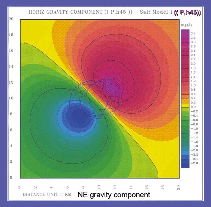
tance X=2R from the center of the sphere of radius R. The
                                                                            apparent gravity doublet and GG triplet patterns encoun-
                                                                            tered in the borehole are similar to the patterns of gravity gra-
                                                                            dient profiles that would be observed on the surface. Thus,
                                                                            interpretation techniques developed and used for borehole
                                                                            gravity and gravity gradient data can be extended and used
                                                                            for surface gravity gradient data interpretation. Overall, expe-
                                                                            rience with interpretation of borehole gravity data can be
                                                                            valuable for the interpretation of surface gravity gradient pro-
                                                                            file and map data.

                                                                            Conclusions. Gravity gradients (GG) often produce a pattern
                                                                            of complex anomalies that is coordinate-dependent, not nec-
                                                                            essarily reflecting the shape of the underlying sources.
                                                                            Understanding GG anomalies is important in the interpreta-
                                                                            tion of measured data. It is easy to understand the complex
                                                                            pattern of gravity gradients if one considers the fact that they
                                                                            are derivable from the simple gravitational potential, being
                                                                            the directional second derivatives of the potential. In general,
                                                                            for 3D sources producing single bell-shaped potential and ver-
                                                                            tical gravity anomalies, the P,zz gravity gradient component
                                                                            consists of a single anomaly; the P,xz and P,yz components
                                                                            consist of doublet anomalies; the P,xx and P,yy components
                                                                            consist of triplet anomalies; and the P,xy component consists
                                                                            of quadruplet anomalies. Various combinations of GG com-
                                                                            ponents can be used to produce coordinate-independent
                                                                            “invariants” that are simple, easy to interpret, more localized,
                                                                            and more related to the size and shape of the sources. There
                                                                            are also similarities between surface and subsurface (or bore-
Figure 15. Borehole vertical gravity and gravity gradient (apparent den-    hole) variations of certain gravity and gravity gradient com-
sity) profiles due to a sphere of radius R, density contrast ∆ρ. Borehole   ponents. Hence, interpretation methods developed and used
distance X = 2R from the center of the sphere.
                                                                            for borehole gravity data may be applicable or can be extended
Similarities between surface and subsurface gravity and                     to surface GG data interpretation. Certainly past experience
gravity gradients. It is interesting to note that there are simi-           with borehole gravity can be valuable in interpreting surface
larities between surface variations of the horizontal gravity               gravity gradient data.
and GG components and subsurface variations of vertical
gravity and vertical GG (or anomalous apparent density) such                Suggested reading. “Gravity gradiometry resurfaces” by Bell et
as those observed in a borehole. Figures 13 and 14 show exam-               al. (TLE, 1997). “Gravity gradiometry in resource exploration”
ples illustrating these similarities. Figure 13 compares surface            by Pawlowski (TLE, 1998). “The gradient tensor of potential field
variations in the x-y plane of the horizontal gravity compo-                anomalies: Some implications on data collection and data pro-
nent P,y (Figure 3) with subsurface variations in the x-z plane             cessing of maps” by Pedersen and Rasmussen (GEOPHYSICS, 1990).
of vertical gravity due to a spherical source. Figure 14 shows              “Euler deconvolution of gravity tensor gradient data” by Zhang
a similar comparison between surface gravity gradient dif-                  et al. (GEOPHYSICS, 2000). TLE
ference (P,xx – P,yy) and subsurface vertical gravity gradient
or apparent density anomaly, as used in borehole gravity                    Acknowledgments: Parts of this work were conducted while the author was
work, due to the same spherical mass. Vertical profiles in the              employed by Gulf Research and Development, Chevron, and Unocal com-
z direction extracted from the maps on the right-hand sides                 panies. This paper was presented at the SEG75 Annual Meeting in Houston,
of Figures 13 and 14 show the anomalous responses expected                  Texas.
in boreholes and measured in borehole gravity surveys (Figure
                                                                            Corresponding author: afifhsaad@netscape.net
15). In this example, the boreholes are located at a remote dis-

                                                                                                               AUGUST 2006     THE LEADING EDGE    949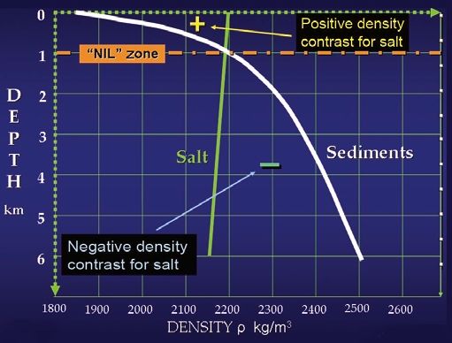
Author Biography

Afif H. Saad is a Geophysical Consultant, specializing in integrated gravity / magnetic /
seismic / geologic interpretation, modeling, magnetic depth estimation, software development,
and training. He has over 25 years of experience in the oil industry, including GULF R&D,
GULF E&P, CHEVRON and UNOCAL Oil Companies. He also held positions with Aero
Service Corp. in Philadelphia and LCT Inc. in Houston as well as in the academia at Cairo
University, Stanford University, and University of Missouri at Rolla. Afif received a Ph.D. in
Geophysics from Stanford University, M.S. in Geology/Geophysics from Missouri School of
Mines-Rolla, and B.Sc. (Honors) Special Geology from Alexandria University, Egypt. He is a
member of SEG, Gravity and Magnetics Committee, and GSH. He was the chairman of the
Houston Potential Fields SIG of GSH from 2000-2004, and an Associate Editor for
GEOPHYSICS – Magnetic Exploration Methods from 1999 – 2005.
You can also read