Surface Potential Surveys Training Manual - G1 Data-logger Version - M. C. Miller Co., Inc. 11640 U.S. Highway 1, Sebastian, FL 32958 Tel: ...
←
→
Page content transcription
If your browser does not render page correctly, please read the page content below
Surface Potential Surveys Training Manual
        – G1 Data-logger Version

               M. C. Miller Co., Inc.
    11640 U.S. Highway 1, Sebastian, FL 32958
    Tel: 772.794.9448 ; Website: www.mcmiller.com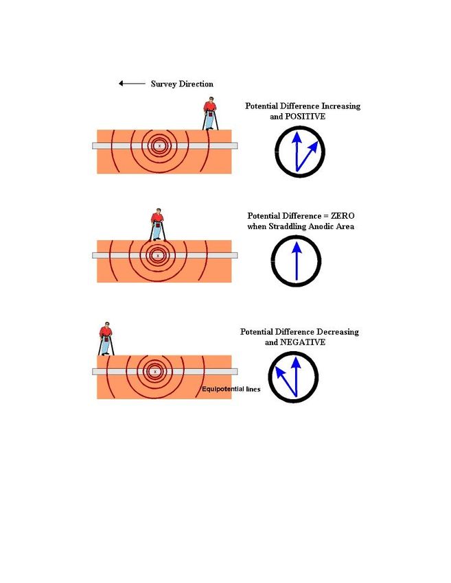
CONTENTS

                                                         Page

Introduction ………………………………………………….. 3

Physical principles …………………………………………... 3

How to setup the G1 for Surface Potential surveys …………    9

Equipment hook-ups ………………………………………… 27

How to perform a Surface Potential survey …………………. 29

                                                                2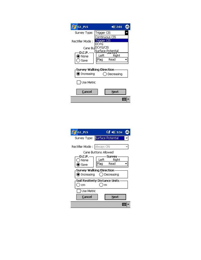
SECTION 1

                              INTRODUCTION

The “Surface Potential (SP)” pipeline survey method, also called the Cell-to-
Cell Potential survey method, is similar to the DCVG survey method, at
least in terms of how the reference electrodes are employed to measure the
difference in potential between two points on the surface of the soil above a
buried pipeline. SP surveys, however, are typically performed on uncoated
pipelines that are not cathodically-protected.

In the case of SP surveys, any localized current flow that gives rise to
potential gradients on the surface of the soil above a buried pipe is due to the
presence of corrosion cells (combinations of anodic and cathodic areas) on
the pipeline, as opposed to impressed current from a CP system which is
responsible for the “signal strength” in the case of DCVG surveys.

In the case of bare pipe, typically only about 10-15 % of the pipe will be
subject to galvanic corrosion and, in addition, typically this small percentage
is made up of small, highly-localized, corrosion areas (anodic areas) that are
randomly-distributed along the length of the pipe. Thus, an “above-the-
ground” survey technique that can accurately locate these isolated areas is
invaluable.

The objective of SP surveys is to locate anodic areas existing along a
segment of pipeline, as evidenced by potential gradient fields presenting
themselves on the surface of the soil directly above the anodic areas. Once
any anodic areas have been located, remedial action can be taken, such as
the installation of “sacrificial” anodes to suppress current flow from the
corroding area, with a view to preventing further external corrosion in that
particular area .

                                  SECTION 2

                         PHYSICAL PRINCIPLES

When current flows onto (or away from) a localized area on a buried-
pipeline, a voltage gradient field presents itself on the surface of the soil
directly above the localized area.

                                                                                3
In the case where current is flowing onto a pipeline at some localized area,
that localized area is considered a cathodic area and the voltage gradient
field on the soil above the pipe will have a negative polarity. The largest
negative potential will exist directly above the anomaly and the negative
potential will decrease in magnitude to remote earth potential with distance
away from the pipe.
The opposite is true in the case where current is flowing away from an
isolated (localized) area on a buried-pipeline. In this case, the area is
considered an anodic area and the voltage gradient field presenting itself on
the surface of the soil above the pipe will have a positive polarity. The
largest positive potential will exist directly above the anodic area and the
positive potential will decrease in magnitude to remote earth potential with
distance away from the pipe.
Since corrosion occurs on an uncoated buried pipeline via the development
of “corrosion cells”, both anodic and cathodic areas must exist
simultaneously. The current flowing away from the anodic area will be
collected by the cathodic area and the return path for the current will be the
pipeline itself.
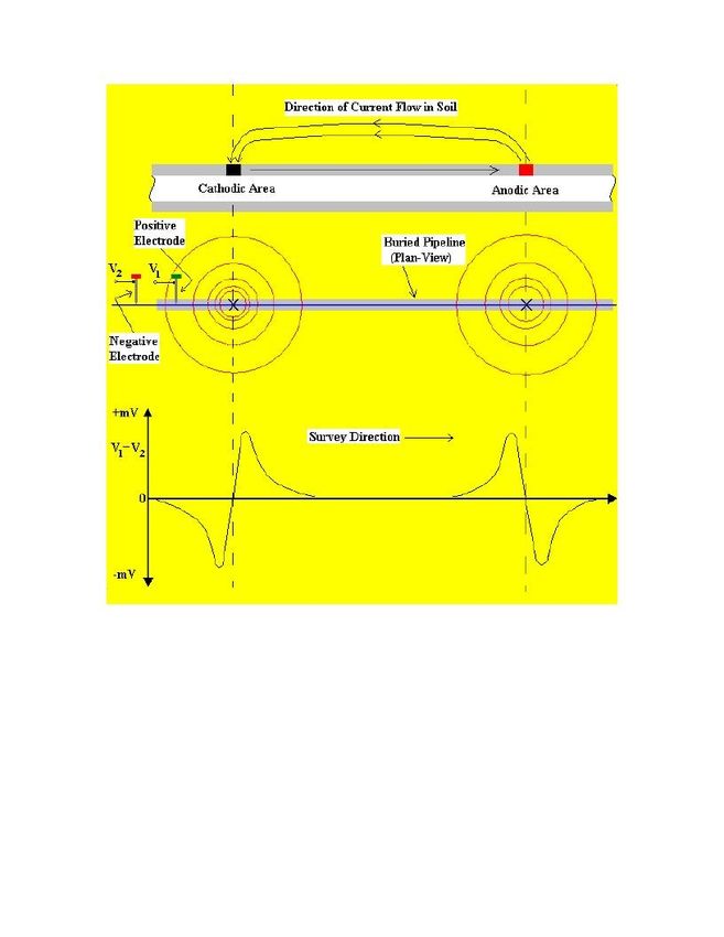
This situation is illustrated schematically in Figure 1 below (top diagram).
4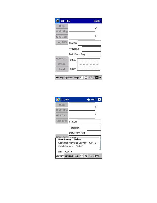
Figure 1:   In-Line method of conducting SP surveys. Soil-to-
            soil potential difference readings are plotted in the bottom
            diagram against the position along the pipeline of the
            center point between the reference electrodes

                                                                           5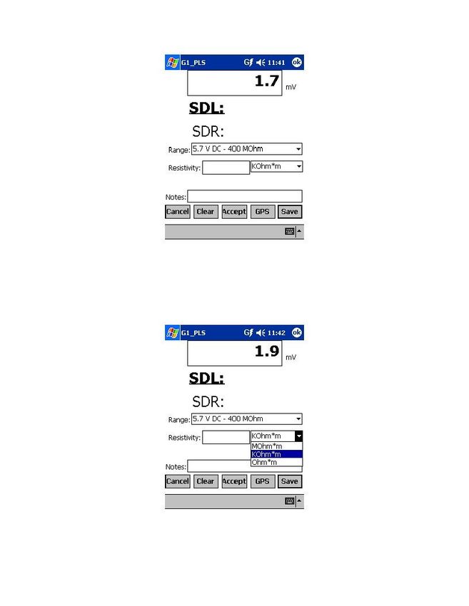
In-Line SP Survey Method

One way to perform a SP pipeline survey is to use the, so-called, “In-Line”
method. In this case, the reference electrodes are both positioned over the
pipe and their separation is kept fixed as the operator, or operators in the
case of large electrode spacings (for example, a 20 feet spacing), walks
down the length of the pipeline section. With a view to detecting localized
anodic areas and accurately measuring the longitudinal voltage profile, the
survey needs to be close-interval in nature.

With the electrodes positioned as illustrated in Figure 1, i.e., with the
positive data-probe leading, when cathodic and anodic areas are
encountered, the polarity of the longitudinal voltage (V¹ minus V²) switches
from negative to positive, in the case of isolated cathodic areas, while in the
case of isolated anodic areas, the polarity switches from positive to negative
as the voltage gradient fields are traversed.

The (longitudinal voltage) polarity switching phenomenon is explained with
reference to Figure 2 below.

For the case of a localized anodic area, the potential gradient on the surface
is positive and, so, when the positive data-probe enters the gradient field, a
positive potential difference will be measured, relative to the zero potential
difference measured with both data-probes positioned outside the gradient
field. The potential difference measured between the probes will continue to
increase, as the data-probes advance into the gradient field, and will go
through a maximum value before dropping through zero (as the data-probes
straddle the epicenter of the anodic area) and becoming negative. After
going through a maximum negative value, the potential difference measured
between the probes will decrease (staying negative) and eventually become
zero again with both data-probes positioned on the far side of the potential
gradient field. This type of longitudinal voltage profile is illustrated in
Figure 1.

It should be noted that the nuances of the profile shown in Figure 1 will only
be observed if the survey is close interval in nature (relative to the size of the
potential gradient field).

                                                                                  6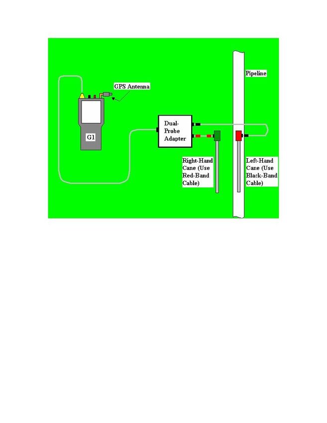
Figure 2:   In-Line SP Survey Method.

            Illustration is for the case of transiting a localized ANODIC
            area with the lead data-probe being the positive probe, in
            which case the polarity of the longitudinal voltage switches
            from positive to negative as the operator walks through the
            voltage gradient field.

                                                                        7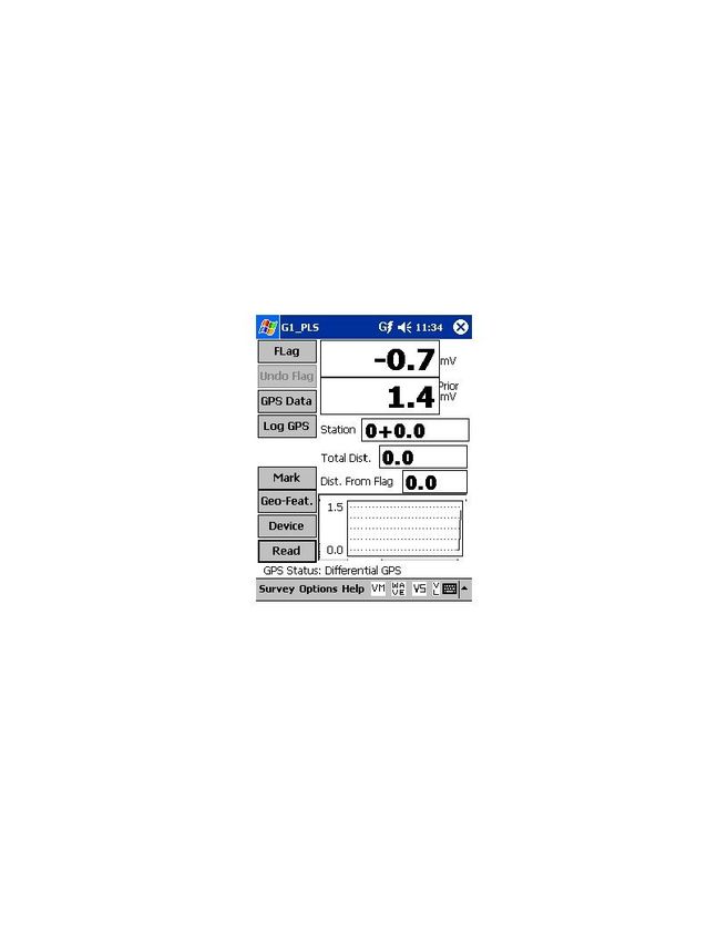
Anodic Area “Severity” Factor:

In addition to locating anodic areas, there is interest in determining some
sort of “severity factor” for each location.

However, unlike in the case of DCVG surveys which utilize a known “signal
strength”, i.e., the IR drop in the soil in the vicinity of the anomaly, there is
no directly measurable “signal strength” in the case of Surface Potential
surveys.

Consequently, some other approach is required to come up with a “severity
factor”.

At the present time, the specification upon which our software is currently
based calls for the generation of a “Corrosion Factor” value for each
“marked” anodic location. The calculation is as follows:

Corrosion Factor = [Maximum longitudinal voltage reading logged on
either side of the SP anomaly (within 2 reading intervals of the “marking”
location)] / [Soil resistivity in the vicinity of the SP anomaly]

Since the magnitude of the current flowing away from an anodic area
correlates with the rate of corrosion in that area, factoring in soil resistivity
makes sense, if we’re trying to get a handle on the rate of corrosion for a
given magnitude of voltage gradient. For instance, for a given magnitude of
voltage gradient on the surface, the corrosion rate will be higher (current
flow away from the pipe will be larger) if the soil resistivity in the area is
relatively small. Conversely, for the same magnitude of voltage gradient on
the surface, the corrosion rate will be lower (current flowing away from the
pipe will be smaller) if the soil resistivity in the area is relatively large.

Another approach regarding Corrosion Factor determination would be to use
the sidedrain readings, which are a direct measure of the gradient field
magnitude, as the numerator in the Corrosion Factor calculation, as opposed
to the “maximum longitudinal voltage” whose value is subject to data-probe
placement, relative to the potential gradient field.

                                                                                    8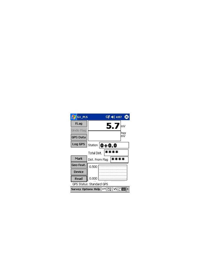
SECTION 3

           HOW TO SET UP THE G1 DATA-LOGGER FOR
                SURFACE POTENTIAL SURVEYS

The following section outlines the steps required to setup the G1 data-logger
to participate in Surface Potential survey applications. The setup process
establishes the conditions of the particular survey about to be performed and
identifies the section of pipeline that is about to be examined by the Surface
Potential application. The setup process also establishes a file in which the
voltage recordings (survey data) will be stored. At the completion of the
survey, Surface Potential survey data can then be retrieved by a PC that is in
communication with the data-logger by accessing the file in which the
survey data are stored.

Step 1:
Switch on the G1 by pressing the power button (red key on keyboard).
Assuming that the battery pack is charged, the screen will light up and will
display the “home” screen (“Today” screen), in the case of the Q100 units,
and the desktop screen, in the case of the Q200 units.

The startup screens for the Q100 and the Q200 units are illustrated below:
Q100 Units:

                                                                               9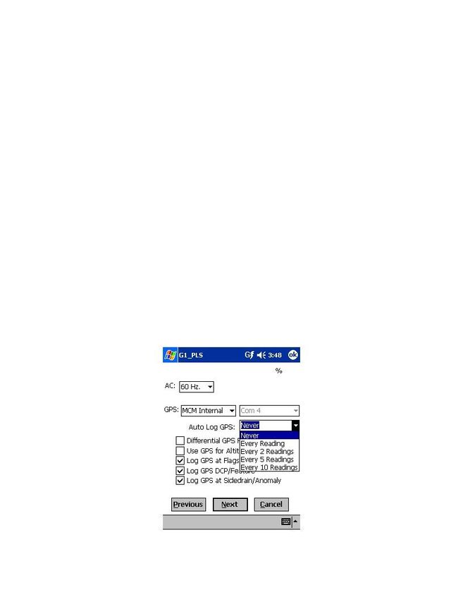
Q200 Units:

Step 2:
In the case of the Q100 units, tap on the “Start” button on the “Home”
screen. This will pull up the main menu.

Step 3:
In the case of the Q100 units, tap on the G1 PLS button on the main menu.
In the case of the Q200 units, double-tap on the G1PLS icon on the desktop
or tap on the start icon (bottom left-hand corner of desktop), tap on the
“Programs” button and tap on the G1PLS button.

In either case (Q100 or Q200 units), the survey screen shown below will be
displayed.

Note: In the case of the Q200 units, the menu items are arrayed along the
top of the screen.

                                                                            10
Step 4:
Tap on “Survey” in the menu bar along the bottom of the above screen. The
screen shown below will appear.
Under “Survey” there are several options. If this is a new survey, not a
continuation of a previous survey, tap on “New Survey”. The screen shown
below will appear.
11Step 6:
Enter a “filename” for the Survey.
Note: This is an important step as the filename is used to identify the survey
and, also, recorded data (voltages) will be stored in this named file for future
retrieval. It is highly recommended that a protocol be established for
selecting Survey Filenames. Critical information should be included in the
filename, such as pipeline company’s name, city or state in which the
pipeline is located, pipeline number and section of pipeline number under
survey. The protocol developed should be applied consistently for each
survey.
For example, let’s assume that pipeline company XYZ has a pipeline located
in Texas and that the pipeline is identified as pipeline 12 and a survey is
being performed on section 085 of this pipeline. A good filename for this
survey would be:
XYZ TX 12 085 SP
When this data file is later accessed, with this filename we know the name of
the pipeline owner, we know the state in which the pipeline is located, we
know the pipeline number, we know the section number of the pipeline that
was surveyed and we know that it was a SP survey.
12Note: You will not be permitted to use invalid characters, such as
slashes( / or \ ), as part of a filename. You will be alerted if you try to
use any invalid characters.
Step 7:
Tap once on the OK button. The screen shown below will appear.
Step 8:
Select “Survey Type”.
The 5 available “survey types” can be seen by tapping on the pull-down list
arrow in the “Survey Type” box as shown on the screen below.
13Tap on “Surface Potential” to select a Surface Potential survey type. The
screen shown below will appear.
14Step 9:
Select Rectifier Mode.
A menu option is not available for “Rectifier Mode”, in the case of Surface
Potential surveys, as such surveys are conducted on non cathodically-
protected pipe.
Step 10:
Make “Cane Button” Functionality Choices
Typically, for Surface Potential surveys, you would “trigger” voltage
recordings using either the positive (green-handled) reference electrode data-
probe or the negative (red-handled) reference electrode data-probe. In the
case where an “in-line” survey is to be performed by two crew members
(one holding the positive electrode (green-handled data-probe), the other
holding the negative electrode (red-handled data-probe), the choice of which
push-button switch to designate as the “trigger” for readings will depend on
which data-probe the crew member operating the G1 is holding. If the G1
operator holds the red-handled (negative) data-probe, the selection should be
“read flag” in the “Survey” category and, if the G1 operator is holding the
green-handled (positive) data-probe, the selection should be “flag read”. In
either case, the crew member who is not the G1 operator could use his push-
button switch to designate the location of survey flags.
You can also use either cane button when recording voltages at D.C.P.’s
(data collection points (devices)) to “save” a device reading, as opposed to
tapping on the “save” button on the screen.
Note: When “Marking” SP anomalies (see Section 5), the cane push-button
functionality becomes “accept”, regardless of whether “save” or “none” is
selected here.
Step11a:
Select Walking Direction
On the Setup 1 of 5 screen, you should indicate whether station numbers will
be increasing or decreasing as you proceed in the survey direction by
tapping on either the “Increasing” or “Decreasing” radio button in the
“Survey Walking Direction” field.
15Step 11b:
Select the length units for your “Soil Resistivity” measurements.
As indicated in the Surface Potential Survey Training Manual, you have the
option to manually enter a value for soil resistivity measured at the location
of a “marked” SP anomaly, which will allow the software to calculate a
“Corrosion Factor”. The units “Ω.cm” or “Ω.m” for soil resistivity that will
appear on the SP anomaly “marking” screen, for your manual data entry,
will depend on your selection here in the “Soil Resistivity Distance Units”
field (cm or m)
Step 11c:
Make selection of “Metric” units if required.
By checking off the box labeled “Metric”, the reading interval (distance
between voltage recordings) and the survey flag internal (survey flag
spacing) will be displayed in meters, as opposed to feet.
Tap on the “Next” button on the above screen.
Step 12:
Select GPS Type
By tapping on the pull-down-list arrow button in the “GPS:” field, you can
select the type of GPS unit you will be using (if any) from the list shown
below.
16As can be seen from the above screen, there are 5 choices for “GPS Type”:
None: This means that a GPS receiver is not being used
MCM External: This means that an external MCM GPS Accessory is
being used
NMEA: This means that an NMEA 0183 compatible GPS
receiver is being used
Manual: This means that location data will be entered manually
when the GPS button is pressed on the survey screen
during a SP survey.
MCM Internal: This means that the G1’s internal GPS unit will be used
(a Garmin (Model 15L) WAAS-enabled receiver)
Select the appropriate choice by tapping on your selection.
When using an external GPS unit, you need to select the Com Port that
you’ll be using on the G1 (see above screen). The connector terminal on the
left-hand side of the data-logger (facing the bottom side) is the COM 1 Port
and the terminal on the right-hand side is the COM 4 Port. It is
recommended that you select the COM 4 Port for your external GPS unit in
order to avoid potential conflicts with ActiveSync which uses COM 1.
17Step 13:
Select GPS Options:
After selecting the GPS Receiver Type and COM Port, choices need to be
made regarding GPS Options (see screen below).
If a GPS accessory has been selected for use with the data-logger for a
particular Surface Potential survey, all, or some of the functions available
can be enabled (box ticked). A box can be “ticked” or “unticked” by tapping
inside the box. The GPS options available are as follows:
Differential GPS Required:
This box should be ticked if you only want differentially-corrected GPS
position data to be logged by the data-logger. If this box is left unticked, it
means that you will allow the G1 data-logger to log either standard GPS
position data or differentially-corrected GPS position data.
Note: Logging “Standard” GPS position data is usually better than having
no data logged at all, which would be the case if you checked this box and
for some reason your GPS receiver was not outputting differentially-
corrected position data. Consequently, it may be preferable to leave this box
unchecked, unless it is imperative that you exclusively log differentially-
corrected GPS position data.
18Use GPS Altitude:
If this box is ticked, altitude data will be included with the position data
whenever GPS data is logged. (Note: Altitude data on some GPS units is not
particularly accurate in survey applications).
Log GPS at Flags:
If this box is ticked, GPS position data will be logged automatically at flags
when either the flag button is tapped (directly on the Survey screen) or when
the push-button on the designated “flag cane” is pressed.
Log GPS at DCP/Feature:
If this box is ticked, GPS position data will be logged automatically at
“Devices” or “Geo-Features” when either the “Device” button is tapped on
the Survey screen and a “Device” reading is logged or when the “Geo-Feat.”
button is tapped on the Survey screen and a geo-feature is registered.
Log GPS at Sidedrain/Anomaly:
If this box is ticked, GPS location data will be logged automatically when
SP anomalies are “marked”.
Auto Log GPS:
By tapping on the drop down menu button in the “Auto Log GPS” field, the
selections available will be displayed as indicated below.
19By selecting one of these options, you can elect to have the GPS position
data logged automatically at every survey reading, at every second reading,
at every fifth reading, at every tenth reading, or not at all (never) at survey
readings.
Step 14:
Finally on the above screen, select the electricity supply operating frequency
of the country in which you are performing the surveys (60Hz or 50Hz). For
the U.S., select 60Hz.
Tap on the “Next” button on the above screen. The screen shown below will
appear.
Step 15:
Enter Pipeline Name and Survey Starting Location
Provide the Name of the Pipeline:
By tapping in the field labeled “Name of P/L”, you can type in the pipeline
name. Note: This is not the same as the filename for the Surface Potential
survey that was selected back at Step 6. This is the actual name of the
pipeline.
20Provide the Valve Segment Identification Number:
By tapping in the field labeled “Valve Segment”, you can type in the valve
segment name or number (if known).
Provide the Starting Location:
Provide the Starting Location for the Survey
You can select to have location information displayed on the survey screen
as station number, feet or milepost (station number, meters or kilometers for
the metric case).
Whichever selection you make here will determine how you enter your
starting location information.
For example, if your pipeline locations are represented by station numbers,
you would select “Station Number” from the drop down list and you would
enter a starting location for the survey in the form of a station number. [If
you do not know the station number where you’re beginning your survey,
enter 0+0.0].
As an example, if you are working on pipeline ABC within valve segment
45 and you are about to begin a Surface Potential survey at station number
12+00.0, your screen would be as shown below.
21Step 16:
Select Voltage Recording Interval (Distance Between Recordings)
By tapping in the field on the above screen labeled “Distance Per Reading”,
you can type in the voltage reading interval (distance in feet (or in meters for
the metric case) expected between recordings) for the Surface Potential
survey.
Step 17:
Select Survey Flag Interval (Distance Between Survey Flags)
By tapping in the box on the above screen labeled “Distance Between
Flags”, you can type in the survey flag interval (distance between survey
flags in feet, or in meters for the metric case) for the section of pipeline
being measured. Typically, survey flags are located at 100 feet intervals.
Step 18:
Select the maximum permissible error between the actual number of
recordings made between 2 survey flags and the expected number of
recordings.
22By tapping in the field labeled, “CIS Flag Read Count %”, you can type in
the maximum permissible error. For example, the maximum permissible
error is indicated as 20% on the above screen. If the recording interval is
expected to be 5.0 feet and the survey flag separation is 100 feet, that means
that 20 recordings are expected. If, however, only 15 recordings are
actually made between survey flags, an error window will appear on the
screen, since there is a 25% difference between the expected and actual
number of recordings made. No error window will appear if the difference
is less than 20% for this example, ie, you could have a minimum of 16
recordings and a maximum of 24 recordings between survey flags to stay
within the 20% (max.) error allowance.
Step 19:
Select whether or not you would like the recordings to be uniformly spaced
between survey flags, in cases where less than or greater than 20 recordings
are made.
By tapping in the box labeled, “Auto Pacing Mode”, and inserting a tick in
the box, you will enable the data-logger to automatically adjust the actual
recordings and space them evenly over the flag spacing distance, regardless
of the actual number of recordings made. Again, enabling this selection is
recommended.
Tap on the Next button on the above screen. The screen shown below will
appear.
23Step 20:
Provide the Work Order Number for the Surface Potential survey.
By tapping in the field on the above screen labeled, “Work Order #”, you
can type in the work order number for the SP survey.
Step 21:
Provide Your Name.
By tapping in the field labeled, “Technician Name”, you can type in your
name or the name of your supervisor. If you use your supervisor’s name
here, you might add your own name in the Comments Section.
Step 22:
Provide Comments.
By tapping in the field labeled, “Comments/Description”, you can enter any
comments you might have regarding the survey (perhaps weather conditions,
soil conditions etc.).
Also shown on the above screen are the Survey (File) Name and the Survey
Start Date and Time.
24Note: Do not attempt to change the File Name indicated here as this
identification will be required by the ProActive software to transfer
your Surface Potential survey data to your PC.
Tap in the Next button on the above screen. The screen shown below will
appear.
Step 23:
Select Voltmeter Settings
Select the “Read Mode”:
SP surveys are typically performed on pipelines that are not cathodically-
protected with impressed current from rectifier sources and so the
appropriate choice of “Read Mode” would be “Single Read”, i.e., “On-Off
Pair” read modes are not appropriate, since rectifier current interruption is
not a factor.
Select the “Range”:
As can be seen by viewing the drop down menu in the “Range” field, a
number of selections are possible.
25The fastest response setting is the 5.7V/400MΩ setting (~80ms response
time), however, the noise level on this setting is ±5mV, which could make
small anomalies difficult to detect.
Lower noise level settings (±1mV noise level)) can be selected, such as the
40mV or 400mV settings to increase sensitivity, however, please note that
the speed of response on these settings is around 1 sec.
Step 24:
Pull-up “Active” Survey Screen
By tapping on the “OK” button on the Voltmeter Settings screen, the
“active” Survey screen would appear and you would be ready to
proceed with your SP survey.
An example starting “active” Survey screen is shown below.
26As SP voltages are recorded by the G1 data-logger, the “Distance From
Start” (total distance from the start of the survey) parameter will increase in
increments of 5.0 feet, or whatever the “Distance Per Reading” value was
that was entered back at Step 16. (Distances would be in meters if the metric
option had been selected).
Also, the “Distance From Known Station” parameter will increase in the
same increments as voltages are recorded. The difference in this case,
however, will be that when a known station is registered, this distance
parameter will begin again at zero. In other words, this will show the
distance you are assumed by the G1 data-logger to have traveled from the
last known station that you encountered (and registered).
You are now ready to perform a Surface Potential survey.
SECTION 4
EQUIPMENT HOOK-UPS
The G1 data-logger, data-probe and data-probe cable hook-ups for Surface
Potential surveys using M. C. Miller equipment are illustrated in Figure 3
below.
As can be seen from Figure 3, two reference electrode data-probes are
illustrated, a RED-handled data-probe and a GREEN-handled data-probe.
These data-probes, which will be placed on the soil above the pipeline in
either the “Perpendicular” or the “In-Line” configuration (see Section 2),
have push button switches on top of the handles so that the operator can
“trigger” voltage recordings at each of the survey measurement locations
and can also designate the locations of survey flags (see Section 3).
The reference electrode data-probes are connected as shown to the “input”
terminals of the dual-probe adapter and the “output” terminal of the adapter
is connected to the 5-pin socket on the top side of the G1 data-logger.
27Figure 3
NOTE: The red-handled cane is connected to the dual probe adapter via a
“black-band” cable while the green-handled cane is connected to the dual-
probe adapter via a “red-band” cable. This results in the reference electrode
of the red-handled data-probe connecting to the negative side of the data
logger’s voltmeter and the reference electrode of the green-handled data-
probe connecting to the positive side of the voltmeter. The red-band and the
black-band cables can be connected to either one of the dual-probe adapter’s
“input” terminals.
Consequently, the data-logger’s voltmeter will measure the potential at the
location of the green-handled (positive) data-probe minus the potential at the
location of the red-handled (negative) data-probe.
28SECTION 5
HOW TO PERFORM A SURFACE POTENTIAL SURVEY
5. 1 How to carry the test equipment during a SP survey
With the equipment connected as shown in Figure 3 (Section 4), and the G1
data-logger “setup” as described in Section 3, you are ready to perform a SP
survey.
To make a pipeline survey more manageable, MCM has developed a special
“belt pack” which allows the G1 to be carried around the waist area in a
“hands-free” fashion.
With the belt pack assembly, the G1 sits on a tray at waist level allowing the
operator to view the screen at all times and to make any selections required
by tapping on the screen. Also, the dual-probe adapter shown in Figure 3, is
attached to the underside of the tray, allowing convenient (5 pin cable)
connection of the adapter’s “output” to the G1.
5. 2 How to locate and “mark” SP anomalies
The objective in SP surveys is to locate anodic areas, i.e., areas on the buried
pipe where current is “leaving” the pipe. As discussed in Section 2, such
areas can be located by observing a polarity switch in the recorded “in-line”
(or longitudinal) voltage. As also discussed in Section 2, the nature of the
polarity switch (i.e., positive-to-negative, or negative-to-positive) depends
on whether the lead data-probe is the “positive” or the “negative” probe.
For the case where the “positive” data-probe is leading (i.e., leading with the
green-handled data-probe), since the potential gradient on the surface is
positive over an anodic area, a positive potential difference will be
measured, as a gradient field is entered, relative to the zero potential
difference measured with both data-probes positioned outside the gradient
field. The potential difference measured between the probes will continue to
increase, as the data-probes advance into the gradient field, and will go
through a maximum value before dropping through zero (as the data-probes
straddle the epicenter of the anodic area) and becoming negative. After
going through a maximum negative value, the potential difference measured
29between the probes will decrease (staying negative) and eventually become
zero again with both data-probes positioned on the far side of the potential
gradient field.
Consequently, in this case, the polarity switch would be positive-to-negative
as the anodic area is traversed. The opposite polarity switch would be
observed if the lead data-probe was the red-handled (negative) probe.
In order to make the process of determining polarity switches easier, the
survey screen displays the prior reading (including its polarity) in addition to
displaying the current SP reading, as shown in the screen below.
By fine-tuning the location of the epicenter of the anomaly, i.e., by
straddling the epicenter with the data-probes and reading (close to) zero mV,
the anomaly can be “marked”.
To do so, you would tap on the “Mark” button on the survey screen which
would pull up the screen shown below.
30You are being given the opportunity to manually enter a value for the soil
resistivity measured in the vicinity of the anomaly. As discussed in Section
2, the software will use this value in its calculation of “Corrosion Factor” for
the anomaly.
31As indicated in the above screen, you can select the units (MΩ.m, KΩ.m or
Ω.m) for your resistivity value [or MΩ.cm, KΩ.cm or Ω.cm, if the “cm”
length unit was selected during setup].
Also, you are being given the opportunity to record the left and right
sidedrain readings.
When you have the data-probes positioned for the left sidedrain reading
(SDL), you would tap on the “Accept” button which would result in the mV
reading being displayed in the SDL field as indicated in the screen below.
Next, you would position the data-probes for the right sidedrain reading
(SDR), and you would tap again on the “Accept” button which would result
in the mV reading being displayed in the SDR field as indicated in the
screen below.
Note: Alternatively to tapping on the “Accept” button on the screen, you
could press the push-button switch on either data-probe handle to “accept”
the SDL and SDR readings.
32Finally, you would tap on the “Save” button which would result in all of the
data associated with the “marking” process being saved. This would return
you to the SP survey screen and you would continue with the survey.
For information on copying SP survey data to ProActive for graphical report
generation, etc., please consult the ProActive Training Manual.
33You can also read