MAGNETISM AND MATTER Chapter Five - ncert
←
→
Page content transcription
If your browser does not render page correctly, please read the page content below

Chapter Five

MAGNETISM AND
MATTER

       5.1 INTRODUCTION
       Magnetic phenomena are universal in nature. Vast, distant galaxies, the
       tiny invisible atoms, humans and beasts all are permeated through and
       through with a host of magnetic fields from a variety of sources. The earth’s
       magnetism predates human evolution. The word magnet is derived from
       the name of an island in Greece called magnesia where magnetic ore
       deposits were found, as early as 600 BC. Shepherds on this island
       complained that their wooden shoes (which had nails) at times stayed
       struck to the ground. Their iron-tipped rods were similarly affected. This
       attractive property of magnets made it difficult for them to move around.
           The directional property of magnets was also known since ancient
       times. A thin long piece of a magnet, when suspended freely, pointed in
       the north-south direction. A similar effect was observed when it was placed
       on a piece of cork which was then allowed to float in still water. The name
       lodestone (or loadstone) given to a naturally occurring ore of iron-
       magnetite means leading stone. The technological exploitation of this
       property is generally credited to the Chinese. Chinese texts dating 400
       BC mention the use of magnetic needles for navigation on ships. Caravans
       crossing the Gobi desert also employed magnetic needles.
           A Chinese legend narrates the tale of the victory of the emperor Huang-ti
       about four thousand years ago, which he owed to his craftsmen (whom

                                2019-20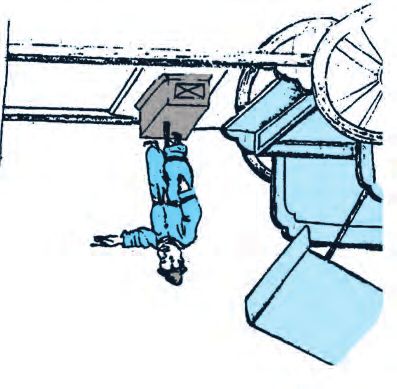
Physics
                                            nowadays you would call engineers). These ‘engineers’
                                            built a chariot on which they placed a magnetic figure
                                            with arms outstretched. Figure 5.1 is an artist’s
                                            description of this chariot. The figure swiveled around
                                            so that the finger of the statuette on it always pointed
                                            south. With this chariot, Huang-ti’s troops were able
                                            to attack the enemy from the rear in thick fog, and to
                                            defeat them.
                                                 In the previous chapter we have learned that moving
                                            charges or electric currents produce magnetic fields.
                                            This discovery, which was made in the early part of the
                                            nineteenth century is credited to Oersted, Ampere, Biot
                                            and Savart, among others.
                                                 In the present chapter, we take a look at magnetism
 FIGURE 5.1 The arm of the statuette
                                            as a subject in its own right.
mounted on the chariot always points
south. This is an artist’s sketch of one         Some of the commonly known ideas regarding
   of the earliest known compasses,         magnetism are:
        thousands of years old.             (i) The earth behaves as a magnet with the magnetic
                                                field pointing approximately from the geographic
                                                south to the north.
                        (ii) When a bar magnet is freely suspended, it points in the north-south
                              direction. The tip which points to the geographic north is called the
                              north pole and the tip which points to the geographic south is called
                              the south pole of the magnet.
                        (iii) There is a repulsive force when north poles ( or south poles ) of two
                              magnets are brought close together. Conversely, there is an attractive
                              force between the north pole of one magnet and the south pole of
                              the other.
                        (iv) We cannot isolate the north, or south pole of a magnet. If a bar magnet
                              is broken into two halves, we get two similar bar magnets with
                              somewhat weaker properties. Unlike electric charges, isolated magnetic
                              north and south poles known as magnetic monopoles do not exist.
                        (v) It is possible to make magnets out of iron and its alloys.
                              We begin with a description of a bar magnet and its behaviour in an
                        external magnetic field. We describe Gauss’s law of magnetism. We then
                        follow it up with an account of the earth’s magnetic field. We next describe
                        how materials can be classified on the basis of their magnetic properties.
                        We describe para-, dia-, and ferromagnetism. We conclude with a section
                        on electromagnets and permanent magnets.

                       5.2 THE BAR MAGNET
                       One of the earliest childhood memories of the famous physicist Albert
                       Einstein was that of a magnet gifted to him by a relative. Einstein was
                       fascinated, and played endlessly with it. He wondered how the magnet
                       could affect objects such as nails or pins placed away from it and not in
 174                   any way connected to it by a spring or string.

                                            2019-20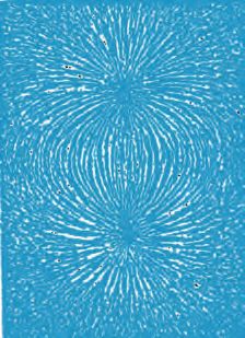
Magnetism and
                                                                         Matter
    We begin our study by examining iron filings sprinkled on a sheet of
glass placed over a short bar magnet. The arrangement of iron filings is
shown in Fig. 5.2.
    The pattern of iron filings suggests that the magnet has two poles
similar to the positive and negative charge of an electric dipole. As
mentioned in the introductory section, one pole is designated the North
pole and the other, the South pole. When suspended freely, these poles
point approximately towards the geographic north and south poles,
respectively. A similar pattern of iron filings is observed around a current
carrying solenoid.

5.2.1 The magnetic field lines
The pattern of iron filings permits us to plot the magnetic field lines*. This is   FIGURE 5.2 The
shown both for the bar-magnet and the current-carrying solenoid in arrangement of iron
Fig. 5.3. For comparison refer to the Chapter 1, Figure 1.17(d). Electric field filings surrounding a
lines of an electric dipole are also displayed in Fig. 5.3(c). The magnetic field   bar magnet. The
lines are a visual and intuitive realisation of the magnetic field. Their            pattern mimics
properties are:                                                                   magnetic  field lines.
                                                                                  The pattern suggests
(i) The magnetic field lines of a magnet (or a solenoid) form continuous
                                                                                  that the bar magnet
     closed loops. This is unlike the electric dipole where these field lines
                                                                                  is a magnetic dipole.
     begin from a positive charge and end on the negative charge or escape
     to infinity.
(ii) The tangent to the field line at a given point represents the direction of
     the net magnetic field B at that point.

     FIGURE 5.3 The field lines of (a) a bar magnet, (b) a current-carrying finite solenoid and
         (c) electric dipole. At large distances, the field lines are very similar. The curves
                           labelled i and ii are closed Gaussian surfaces.

* In some textbooks the magnetic field lines are called magnetic lines of force.
  This nomenclature is avoided since it can be confusing. Unlike electrostatics
  the field lines in magnetism do not indicate the direction of the force on a
  (moving) charge.                                                                                175

                                                   2019-20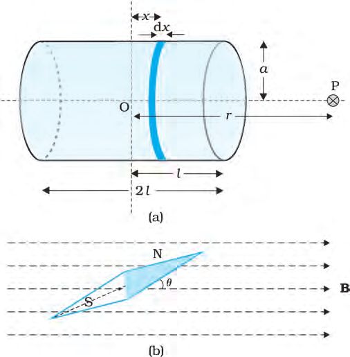
Physics
                         (iii) The larger the number of field lines crossing per unit area, the stronger
                               is the magnitude of the magnetic field B. In Fig. 5.3(a), B is larger
                               around region ii than in region i .
                         (iv) The magnetic field lines do not intersect, for if they did, the direction
                               of the magnetic field would not be unique at the point of intersection.
                               One can plot the magnetic field lines in a variety of ways. One way is
                         to place a small magnetic compass needle at various positions and note
                         its orientation. This gives us an idea of the magnetic field direction at
                         various points in space.

                         5.2.2 Bar magnet as an equivalent solenoid
                         In the previous chapter, we have explained how a current loop acts as a
                         magnetic dipole (Section 4.10). We mentioned Ampere’s hypothesis that
                         all magnetic phenomena can be explained in terms of circulating currents.
                                                        Recall that the magnetic dipole moment m
                                                        associated with a current loop was defined
                                                        to be m = NI A where N is the number of
                                                        turns in the loop, I the current and A the
                                                        area vector (Eq. 4.30).
                                                             The resemblance of magnetic field lines
                                                        for a bar magnet and a solenoid suggest that
                                                        a bar magnet may be thought of as a large
                                                        number of circulating currents in analogy
                                                        with a solenoid. Cutting a bar magnet in half
                                                        is like cutting a solenoid. We get two smaller
                                                        solenoids with weaker magnetic properties.
                                                        The field lines remain continuous, emerging
                                                        from one face of the solenoid and entering
                                                        into the other face. One can test this analogy
                                                        by moving a small compass needle in the
                                                        neighbourhood of a bar magnet and a
                                                        current-carrying finite solenoid and noting
                                                        that the deflections of the needle are similar
                                                        in both cases.
                                                        To make this analogy more firm we
                                                        calculate the axial field of a finite solenoid
  FIGURE 5.4 Calculation of (a) The axial field of a
                                                        depicted in Fig. 5.4 (a). We shall demonstrate
finite solenoid in order to demonstrate its similarity
    to that of a bar magnet. (b) A magnetic needle
                                                        that at large distances this axial field
          in a uniform magnetic field B. The            resembles that of a bar magnet.
             arrangement may be used to                      Let the solenoid of Fig. 5.4(a) consists of
          determine either B or the magnetic            n turns per unit length. Let its length be 2l
               moment m of the needle.                  and radius a. We can evaluate the axial field
                                                        at a point P, at a distance r from the centre O
                         of the solenoid. To do this, consider a circular element of thickness dx of
                         the solenoid at a distance x from its centre. It consists of n dx turns. Let I
                         be the current in the solenoid. In Section 4.6 of the previous chapter we
                         have calculated the magnetic field on the axis of a circular current loop.
                         From Eq. (4.13), the magnitude of the field at point P due to the circular
  176                    element is

                                              2019-20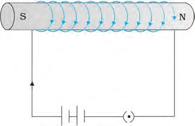
Magnetism and
                                                                        Matter

                µ0n dx I a 2
    dB =                       3
            2[(r − x )2 + a 2 ] 2
   The magnitude of the total field is obtained by summing over all the
elements — in other words by integrating from x = – l to x = + l . Thus,
          µ0nIa 2        l                dx
    B=
            2
                    ∫    −l      [(r − x )2 + a 2 ]3 / 2
    This integration can be done by trigonometric substitutions. This
exercise, however, is not necessary for our purpose. Note that the range
of x is from – l to + l . Consider the far axial field of the solenoid, i.e.,
r >> a and r >> l . Then the denominator is approximated by
                     3
    [(r − x )2 + a 2 ]       2
                                     ≈ r3
                                 l
            µ0 n I a 2
and B =
              2r 3            ∫ dx
                              −l

             µ0 n I 2 l a 2
        =                                                              (5.1)
              2        r3
   Note that the magnitude of the magnetic moment of the solenoid is,
m = n (2 l) I (π a 2 ) — (total number of turns × current × cross-sectional
area). Thus,
          µ0 2m
    B=                                                                  (5.2)
          4π r 3
     This is also the far axial magnetic field of a bar magnet which one may
obtain experimentally. Thus, a bar magnet and a solenoid produce similar
magnetic fields. The magnetic moment of a bar magnet is thus equal to
the magnetic moment of an equivalent solenoid that produces the same
magnetic field.
     Some textbooks assign a magnetic charge (also called pole strength)
+qmto the north pole and –qm to the south pole of a bar magnet of length
2l , and magnetic moment qm(2l). The field strength due to qm at a distance
r from it is given by µ0qm/4πr 2. The magnetic field due to the bar magnet
is then obtained, both for the axial and the equatorial case, in a manner
analogous to that of an electric dipole (Chapter 1). The method is simple
and appealing. However, magnetic monopoles do not exist, and we have
avoided this approach for that reason.

5.2.3 The dipole in a uniform magnetic field
The pattern of iron filings, i.e., the magnetic field lines gives us an
approximate idea of the magnetic field B. We may at times be required to
determine the magnitude of B accurately. This is done by placing a small
compass needle of known magnetic moment m and moment of inertia I
and allowing it to oscillate in the magnetic field. This arrangement is shown
in Fig. 5.4(b).
   The torque on the needle is [see Eq. (4.29)],
   τ=m×B                                                                (5.3)        177

                                                           2019-20
Physics
In magnitude τ = mB sinθ
Here τ is restoring torque and θ is the angle between m and B.
d 2θ
Therefore, in equilibrium I = − mB sin θ
dt 2
Negative sign with mB sinθ implies that restoring torque is in opposition
to deflecting torque. For small values of θ in radians, we approximate
sin θ ≈ θ and get
d 2θ
I ≈ –mB θ
dt 2
d 2θ mB
or, 2
=− θ
dt I
This represents a simple harmonic motion. The square of the angular
frequency is ω 2 = mB/I and the time period is,
I
T = 2π (5.4)
mB
4 π2 I
or B= (5.5)
m T2
An expression for magnetic potential energy can also be obtained on
lines similar to electrostatic potential energy.
The magnetic potential energy Um is given by
U m = ∫ τ (θ )dθ
= ∫ mB sin θ dθ = −mB cos θ
= −m.B (5.6)
We have emphasised in Chapter 2 that the zero of potential energy
can be fixed at one’s convenience. Taking the constant of integration to be
zero means fixing the zero of potential energy at θ = 90°, i.e., when the
needle is perpendicular to the field. Equation (5.6) shows that potential
energy is minimum (= –mB) at θ = 0° (most stable position) and maximum
(= +mB) at θ = 180° (most unstable position).
Example 5.1 In Fig. 5.4(b), the magnetic needle has magnetic moment
6.7 × 10⁻² Am2 and moment of inertia I = 7.5 × 10⁻⁶ kg m2. It performs
10 complete oscillations in 6.70 s. What is the magnitude of the
magnetic field?
Solution The time period of oscillation is,
6.70
T = = 0.67s
10
From Eq. (5.5)
4π 2 I
EXAMPLE 5.1
B= 2
mT
4 × (3.14)2 × 7.5 × 10−6
=
6.7 × 10 –2 × (0.67)2
178 = 0.01 T
2019-20Magnetism and
Matter
Example 5.2 A short bar magnet placed with its axis at 30° with an
external field of 800 G experiences a torque of 0.016 Nm. (a) What is
the magnetic moment of the magnet? (b) What is the work done in
moving it from its most stable to most unstable position? (c) The bar
magnet is replaced by a solenoid of cross-sectional area 2 × 10⁻⁴ m2
and 1000 turns, but of the same magnetic moment. Determine the
current flowing through the solenoid.
Solution
(a) From Eq. (5.3), τ = m B sin θ, θ = 30°, hence sinθ =1/2.
Thus, 0.016 = m × (800 × 10–4 T) × (1/2)
m = 160 × 2/800 = 0.40 A m2
(b) From Eq. (5.6), the most stable position is θ = 0° and the most
unstable position is θ = 180°. Work done is given by
W = U m (θ = 180°) − U m (θ = 0°)
EXAMPLE 5.2
= 2 m B = 2 × 0.40 × 800 × 10–4 = 0.064 J
(c) From Eq. (4.30), ms = NIA. From part (a), ms = 0.40 A m2
0.40 = 1000 × I × 2 × 10⁻⁴
I = 0.40 × 10⁴/(1000 × 2) = 2A
Example 5.3
(a) What happens if a bar magnet is cut into two pieces: (i) transverse
to its length, (ii) along its length?
(b) A magnetised needle in a uniform magnetic field experiences a
torque but no net force. An iron nail near a bar magnet, however,
experiences a force of attraction in addition to a torque. Why?
(c) Must every magnetic configuration have a north pole and a south
pole? What about the field due to a toroid?
(d) Two identical looking iron bars A and B are given, one of which is
definitely known to be magnetised. (We do not know which one.)
How would one ascertain whether or not both are magnetised? If
only one is magnetised, how does one ascertain which one? [Use
nothing else but the bars A and B.]
Solution
(a) In either case, one gets two magnets, each with a north and south
pole.
(b) No force if the field is uniform. The iron nail experiences a non-
uniform field due to the bar magnet. There is induced magnetic
moment in the nail, therefore, it experiences both force and torque.
The net force is attractive because the induced south pole (say) in
the nail is closer to the north pole of magnet than induced north
pole.
(c) Not necessarily. True only if the source of the field has a net non-
zero magnetic moment. This is not so for a toroid or even for a
straight infinite conductor.
(d) Try to bring different ends of the bars closer. A repulsive force in
EXAMPLE 5.3
some situation establishes that both are magnetised. If it is always
attractive, then one of them is not magnetised. In a bar magnet
the intensity of the magnetic field is the strongest at the two ends
(poles) and weakest at the central region. This fact may be used to
determine whether A or B is the magnet. In this case, to see which 179
2019-20Physics
EXAMPLE 5.3
one of the two bars is a magnet, pick up one, (say, A) and lower one of
its ends; first on one of the ends of the other (say, B), and then on the
middle of B. If you notice that in the middle of B, A experiences no
force, then B is magnetised. If you do not notice any change from the
end to the middle of B, then A is magnetised.
5.2.4 The electrostatic analog
Comparison of Eqs. (5.2), (5.3) and (5.6) with the corresponding equations
for electric dipole (Chapter 1), suggests that magnetic field at large
distances due to a bar magnet of magnetic moment m can be obtained
from the equation for electric field due to an electric dipole of dipole moment
p, by making the following replacements:
1 µ
E →B , p → m , → 0
4 πε 0 4π
In particular, we can write down the equatorial field (BE) of a bar magnet
at a distance r, for r >> l, where l is the size of the magnet:
µ0 m
BE = − (5.7)
4 πr 3
Likewise, the axial field (BA) of a bar magnet for r >> l is:
µ0 2m
BA = (5.8)
4 π r3
Equation (5.8) is just Eq. (5.2) in the vector form. Table 5.1 summarises
the analogy between electric and magnetic dipoles.
TABLE 5.1 THE DIPOLE ANALOGY
Electrostatics Magnetism
1/ε0 µ0
Dipole moment p m
Equatorial Field for a short dipole –p/4πε0r 3 – µ0 m / 4π r 3
Axial Field for a short dipole 2p/4πε0r 3 µ0 2m / 4π r 3
External Field: torque p×E m×B
External Field: Energy –p.E –m.B
Example 5.4 What is the magnitude of the equatorial and axial fields
due to a bar magnet of length 5.0 cm at a distance of 50 cm from its
mid-point? The magnetic moment of the bar magnet is 0.40 A m2, the
same as in Example 5.2.
Solution From Eq. (5.7)
EXAMPLE 5.4
µ0m 10 −7 × 0.4 10 −7 × 0.4
BE = = = −7
4 πr3 (0.5)3 0.125 = 3.2 × 10 T
µ0 2m
From Eq. (5.8), B A = 4 π r 3 = 6.4 × 10 −7 T
180
2019-20Magnetism and
Matter
Example 5.5 Figure 5.5 shows a small magnetised needle P placed at
a point O. The arrow shows the direction of its magnetic moment. The
other arrows show different positions (and orientations of the magnetic
moment) of another identical magnetised needle Q.
(a) In which configuration the system is not in equilibrium?
(b) In which configuration is the system in (i) stable, and (ii) unstable
equilibrium?
(c) Which configuration corresponds to the lowest potential energy
among all the configurations shown?
FIGURE 5.5
Solution
Potential energy of the configuration arises due to the potential energy of
one dipole (say, Q) in the magnetic field due to other (P). Use the result
that the field due to P is given by the expression [Eqs. (5.7) and (5.8)]:
µ0 m P
BP = − (on the normal bisector)
4π r 3
µ0 2 mP
BP = (on the axis)
4π r 3
where mP is the magnetic moment of the dipole P.
Equilibrium is stable when mQ is parallel to BP, and unstable when it
is anti-parallel to BP.
For instance for the configuration Q 3 for which Q is along the
perpendicular bisector of the dipole P, the magnetic moment of Q is
parallel to the magnetic field at the position 3. Hence Q3 is stable.
EXAMPLE 5.5
Thus,
(a) PQ1 and PQ2
(b) (i) PQ3, PQ6 (stable); (ii) PQ5, PQ4 (unstable)
(c) PQ6
5.3 MAGNETISM AND GAUSS’S LAW
In Chapter 1, we studied Gauss’s law for electrostatics. In Fig 5.3(c), we
see that for a closed surface represented by i , the number of lines leaving
the surface is equal to the number of lines entering it. This is consistent
with the fact that no net charge is enclosed by the surface. However, in
the same figure, for the closed surface ii , there is a net outward flux, since
it does include a net (positive) charge. 181
2019-20Physics
The situation is radically different for magnetic fields
which are continuous and form closed loops. Examine the
Gaussian surfaces represented by i or ii in Fig 5.3(a) or
Fig. 5.3(b). Both cases visually demonstrate that the
number of magnetic field lines leaving the surface is
balanced by the number of lines entering it. The net
magnetic flux is zero for both the surfaces. This is true
for any closed surface.
KARL FRIEDRICH GAUSS (1777 – 1855)
Karl Friedrich Gauss
(1777 – 1855) He was a
child prodigy and was gifted
in mathematics, physics,
engineering, astronomy
and even land surveying.
The properties of numbers
fascinated him, and in his FIGURE 5.6
work he anticipated major
Consider a small vector area element ∆S of a closed
mathematical development
of later times. Along with
surface S as in Fig. 5.6. The magnetic flux through ÄS is
Wilhelm Welser, he built the defined as ∆φB = B.∆S, where B is the field at ∆S. We divide
first electric telegraph in S into many small area elements and calculate the
1833. His mathematical individual flux through each. Then, the net flux φB is,
theory of curved surface
laid the foundation for the φB = ∑ ∆φ B = ∑ B.∆S = 0 (5.9)
’ all ’ ’ all ’
later work of Riemann.
where ‘all’ stands for ‘all area elements ∆S′. Compare this
with the Gauss’s law of electrostatics. The flux through a closed surface
in that case is given by
q
∑ E.∆S = ε
0
where q is the electric charge enclosed by the surface.
The difference between the Gauss’s law of magnetism and that for
electrostatics is a reflection of the fact that isolated magnetic poles (also
called monopoles) are not known to exist. There are no sources or sinks
of B; the simplest magnetic element is a dipole or a current loop. All
magnetic phenomena can be explained in terms of an arrangement of
dipoles and/or current loops.
Thus, Gauss’s law for magnetism is:
The net magnetic flux through any closed surface is zero.
EXAMPLE 5.6
Example 5.6 Many of the diagrams given in Fig. 5.7 show magnetic
field lines (thick lines in the figure) wrongly. Point out what is wrong
with them. Some of them may describe electrostatic field lines correctly.
Point out which ones.
182
2019-20Magnetism and
Matter
FIGURE 5.7
Solution
(a) Wrong. Magnetic field lines can never emanate from a point, as
shown in figure. Over any closed surface, the net flux of B must
EXAMPLE 5.6
always be zero, i.e., pictorially as many field lines should seem to
enter the surface as the number of lines leaving it. The field lines
shown, in fact, represent electric field of a long positively charged
wire. The correct magnetic field lines are circling the straight
conductor, as described in Chapter 4.
183
2019-20Physics
(b) Wrong. Magnetic field lines (like electric field lines) can never cross
each other, because otherwise the direction of field at the point of
intersection is ambiguous. There is further error in the figure.
Magnetostatic field lines can never form closed loops around empty
space. A closed loop of static magnetic field line must enclose a
region across which a current is passing. By contrast, electrostatic
field lines can never form closed loops, neither in empty space,
nor when the loop encloses charges.
(c) Right. Magnetic lines are completely confined within a toroid.
Nothing wrong here in field lines forming closed loops, since each
loop encloses a region across which a current passes. Note, for
clarity of figure, only a few field lines within the toroid have been
shown. Actually, the entire region enclosed by the windings
contains magnetic field.
(d) Wrong. Field lines due to a solenoid at its ends and outside cannot
be so completely straight and confined; such a thing violates
Ampere’s law. The lines should curve out at both ends, and meet
eventually to form closed loops.
(e) Right. These are field lines outside and inside a bar magnet. Note
carefully the direction of field lines inside. Not all field lines emanate
out of a north pole (or converge into a south pole). Around both
the N-pole, and the S-pole, the net flux of the field is zero.
(f ) Wrong. These field lines cannot possibly represent a magnetic field.
Look at the upper region. All the field lines seem to emanate out of
the shaded plate. The net flux through a surface surrounding the
shaded plate is not zero. This is impossible for a magnetic field.
The given field lines, in fact, show the electrostatic field lines
around a positively charged upper plate and a negatively charged
lower plate. The difference between Fig. [5.7(e) and (f )] should be
EXAMPLE 5.6
carefully grasped.
(g) Wrong. Magnetic field lines between two pole pieces cannot be
precisely straight at the ends. Some fringing of lines is inevitable.
Otherwise, Ampere’s law is violated. This is also true for electric
field lines.
Example 5.7
(a) Magnetic field lines show the direction (at every point) along which
a small magnetised needle aligns (at the point). Do the magnetic
field lines also represent the lines of force on a moving charged
particle at every point?
(b) Magnetic field lines can be entirely confined within the core of a
toroid, but not within a straight solenoid. Why?
(c) If magnetic monopoles existed, how would the Gauss’s law of
magnetism be modified?
(d) Does a bar magnet exert a torque on itself due to its own field?
Does one element of a current-carrying wire exert a force on another
element of the same wire?
(e) Magnetic field arises due to charges in motion. Can a system have
EXAMPLE 5.7
magnetic moments even though its net charge is zero?
Solution
(a) No. The magnetic force is always normal to B (remember magnetic
force = qv × B). It is misleading to call magnetic field lines as lines
184 of force.
2019-20Magnetism and
Matter
(b) If field lines were entirely confined between two ends of a straight
solenoid, the flux through the cross-section at each end would be
non-zero. But the flux of field B through any closed surface must
always be zero. For a toroid, this difficulty is absent because it
has no ‘ends’.
(c) Gauss’s law of magnetism states that the flux of B through any
closed surface is always zero
∫s B .∆s = 0 .
If monopoles existed, the right hand side would be equal to the
monopole (magnetic charge) qm enclosed by S. [Analogous to
Gauss’s law of electrostatics, ∫ B.∆s = µ q
S
0 m where qm is the
(monopole) magnetic charge enclosed by S .]
(d) No. There is no force or torque on an element due to the field
produced by that element itself. But there is a force (or torque) on
an element of the same wire. (For the special case of a straight
wire, this force is zero.)
EXAMPLE 5.7
(e) Yes. The average of the charge in the system may be zero. Yet, the
mean of the magnetic moments due to various current loops may
not be zero. We will come across such examples in connection
with paramagnetic material where atoms have net dipole moment
through their net charge is zero.
5.4 THE EARTH’S MAGNETISM
Earlier we have referred to the magnetic field of the earth. The strength of
the earth’s magnetic field varies from place to place on the earth’s surface;
its value being of the order of 10–5 T.
http://www.ngdc.noaa.gov/geomag/
Geomagnetic field frequently asked questions
What causes the earth to have a magnetic field is not clear. Originally
the magnetic field was thought of as arising from a giant bar magnet
placed approximately along the axis of rotation of the earth and deep in
the interior. However, this simplistic picture is certainly not correct. The
magnetic field is now thought to arise due to electrical currents produced
by convective motion of metallic fluids (consisting mostly of molten
iron and nickel) in the outer core of the earth. This is known as the
dynamo effect.
The magnetic field lines of the earth resemble that of a (hypothetical)
magnetic dipole located at the centre of the earth. The axis of the dipole
does not coincide with the axis of rotation of the earth but is presently
titled by approximately 11.3° with respect to the later. In this way of looking
at it, the magnetic poles are located where the magnetic field lines due to
the dipole enter or leave the earth. The location of the north magnetic pole
is at a latitude of 79.74° N and a longitude of 71.8° W, a place somewhere
in north Canada. The magnetic south pole is at 79.74° S, 108.22° E in
the Antarctica.
The pole near the geographic north pole of the earth is called the north
magnetic pole. Likewise, the pole near the geographic south pole is called 185
2019-20Physics
the south magnetic pole. There is some confusion in the
nomenclature of the poles. If one looks at the magnetic
field lines of the earth (Fig. 5.8), one sees that unlike in the
case of a bar magnet, the field lines go into the earth at the
north magnetic pole (Nm ) and come out from the south
magnetic pole (Sm ). The convention arose because the
magnetic north was the direction to which the north
pole of a magnetic needle pointed; the north pole of
a magnet was so named as it was the north seeking
pole. Thus, in reality, the north magnetic pole behaves
FIGURE 5.8 The earth as a giant like the south pole of a bar magnet inside the earth and
magnetic dipole. vice versa.
Example 5.8 The earth’s magnetic field at the equator is approximately
0.4 G. Estimate the earth’s dipole moment.
Solution From Eq. (5.7), the equatorial magnetic field is,
µ 0m
BE =
4 πr3
We are given that BE ~ 0.4 G = 4 × 10⁻⁵ T. For r, we take the radius of
the earth 6.4 × 10⁶ m. Hence,
EXAMPLE 5.8
4 × 10−5 × (6.4 × 106 )3
m = =4 × 102 × (6.4 × 106)3 (µ0/4π = 10–7)
µ0 / 4 π
= 1.05 × 10²³ A m2
This is close to the value 8 × 10²² A m2 quoted in geomagnetic texts.
5.4.1 Magnetic declination and dip
Consider a point on the earth’s surface. At such a point, the direction of
the longitude circle determines the geographic north-south direction, the
line of longitude towards the north pole being the direction of
true north. The vertical plane containing the longitude circle
and the axis of rotation of the earth is called the geographic
meridian. In a similar way, one can define magnetic meridian
of a place as the vertical plane which passes through the
imaginary line joining the magnetic north and the south poles.
This plane would intersect the surface of the earth in a
longitude like circle. A magnetic needle, which is free to swing
horizontally, would then lie in the magnetic meridian and the
north pole of the needle would point towards the magnetic
north pole. Since the line joining the magnetic poles is titled
with respect to the geographic axis of the earth, the magnetic
meridian at a point makes angle with the geographic meridian.
FIGURE 5.9 A magnetic needle This, then, is the angle between the true geographic north and
free to move in horizontal plane, the north shown by a compass needle. This angle is called the
points toward the magnetic magnetic declination or simply declination (Fig. 5.9).
north-south The declination is greater at higher latitudes and smaller
186 direction.
near the equator. The declination in India is small, it being
2019-20Magnetism and
Matter
0°41′ E at Delhi and 0°58′ W at Mumbai. Thus, at both these places a
magnetic needle shows the true north quite accurately.
There is one more quantity of interest. If a magnetic needle is perfectly
balanced about a horizontal axis so that it can swing in a plane of the
magnetic meridian, the needle would make an angle with the horizontal
(Fig. 5.10). This is known as the angle of dip (also known as inclination).
Thus, dip is the angle that the total magnetic field BE of the earth makes
with the surface of the earth. Figure 5.11 shows the magnetic meridian
plane at a point P on the surface of the earth. The plane is a section through
the earth. The total magnetic field at P
can be resolved into a horizontal
component H E and a vertical
component ZE. The angle that BE makes
with HE is the angle of dip, I.
FIGURE 5.10 The circle is a FIGURE 5.11 The earth’s
section through the earth magnetic field, BE, its horizontal
containing the magnetic and vertical components, HE and
meridian. The angle between BE ZE. Also shown are the
and the horizontal component declination, D and the
HE is the angle of dip. inclination or angle of dip, I.
In most of the northern hemisphere, the north pole of the dip needle
tilts downwards. Likewise in most of the southern hemisphere, the south
pole of the dip needle tilts downwards.
To describe the magnetic field of the earth at a point on its surface, we
need to specify three quantities, viz., the declination D, the angle of dip or
the inclination I and the horizontal component of the earth’s field HE. These
are known as the element of the earth’s magnetic field.
Representing the verticle component by ZE, we have
ZE = BE sinI [5.10(a)]
HE = BE cosI [5.10(b)]
which gives,
ZE
tan I = [5.10(c)]
HE 187
2019-20Physics
WHAT HAPPENS TO MY COMPASS NEEDLES AT THE POLES?
A compass needle consists of a magnetic needle which floats on a pivotal point. When the
compass is held level, it points along the direction of the horizontal component of the earth’s
magnetic field at the location. Thus, the compass needle would stay along the magnetic
meridian of the place. In some places on the earth there are deposits of magnetic minerals
which cause the compass needle to deviate from the magnetic meridian. Knowing the magnetic
declination at a place allows us to correct the compass to determine the direction of true
north.
So what happens if we take our compass to the magnetic pole? At the poles, the magnetic
field lines are converging or diverging vertically so that the horizontal component is negligible.
If the needle is only capable of moving in a horizontal plane, it can point along any direction,
rendering it useless as a direction finder. What one needs in such a case is a dip needle
which is a compass pivoted to move in a vertical plane containing the magnetic field of the
earth. The needle of the compass then shows the angle which the magnetic field makes with
the vertical. At the magnetic poles such a needle will point straight down.
Example 5.9 In the magnetic meridian of a certain place, the
horizontal component of the earth’s magnetic field is 0.26G and the
dip angle is 60°. What is the magnetic field of the earth at this location?
Solution
It is given that HE = 0.26 G. From Fig. 5.11, we have
HE
cos 600 =
BE
EXAMPLE 5.9
HE
BE =
cos 600
0.26
= = 0.52 G
188 (1/2)
2019-20Magnetism and
Matter
EARTH’S MAGNETIC FIELD
It must not be assumed that there is a giant bar magnet deep inside the earth which is
causing the earth’s magnetic field. Although there are large deposits of iron inside the earth,
it is highly unlikely that a large solid block of iron stretches from the magnetic north pole to
the magnetic south pole. The earth’s core is very hot and molten, and the ions of iron and
nickel are responsible for earth’s magnetism. This hypothesis seems very probable. Moon,
which has no molten core, has no magnetic field, Venus has a slower rate of rotation, and a
weaker magnetic field, while Jupiter, which has the fastest rotation rate among planets, has
a fairly strong magnetic field. However, the precise mode of these circulating currents and
the energy needed to sustain them are not very well understood. These are several open
questions which form an important area of continuing research.
The variation of the earth’s magnetic field with position is also an interesting area of
study. Charged particles emitted by the sun flow towards the earth and beyond, in a stream
called the solar wind. Their motion is affected by the earth’s magnetic field, and in turn, they
affect the pattern of the earth’s magnetic field. The pattern of magnetic field near the poles is
quite different from that in other regions of the earth.
The variation of earth’s magnetic field with time is no less fascinating. There are short
term variations taking place over centuries and long term variations taking place over a
period of a million years. In a span of 240 years from 1580 to 1820 AD, over which records
are available, the magnetic declination at London has been found to change by 3.5°,
suggesting that the magnetic poles inside the earth change position with time. On the scale
of a million years, the earth’s magnetic fields has been found to reverse its direction. Basalt
contains iron, and basalt is emitted during volcanic activity. The little iron magnets inside it
align themselves parallel to the magnetic field at that place as the basalt cools and solidifies.
Geological studies of basalt containing such pieces of magnetised region have provided
evidence for the change of direction of earth’s magnetic field, several times in the past.
5.5 MAGNETISATION AND MAGNETIC INTENSITY
The earth abounds with a bewildering variety of elements and compounds.
In addition, we have been synthesising new alloys, compounds and even
elements. One would like to classify the magnetic properties of these
substances. In the present section, we define and explain certain terms
which will help us to carry out this exercise.
We have seen that a circulating electron in an atom has a magnetic
moment. In a bulk material, these moments add up vectorially and they
can give a net magnetic moment which is non-zero. We define
magnetisation M of a sample to be equal to its net magnetic moment per
unit volume:
mnet
M= (5.11)
V
M is a vector with dimensions L–1 A and is measured in a units of A m–1.
Consider a long solenoid of n turns per unit length and carrying a
current I. The magnetic field in the interior of the solenoid was shown to
be given by 189
2019-20Physics
B0 = µ0 nI (5.12)
If the interior of the solenoid is filled with a material with non-zero
magnetisation, the field inside the solenoid will be greater than B0. The
net B field in the interior of the solenoid may be expressed as
B = B0 + Bm (5.13)
where Bm is the field contributed by the material core. It turns out that
this additional field Bm is proportional to the magnetisation M of the
material and is expressed as
Bm = µ0M (5.14)
where µ0 is the same constant (permittivity of vacuum) that appears in
Biot-Savart’s law.
It is convenient to introduce another vector field H, called the magnetic
intensity, which is defined by
B
H= –M (5.15)
µ0
where H has the same dimensions as M and is measured in units of A m–1.
Thus, the total magnetic field B is written as
B = µ0 (H + M) (5.16)
We repeat our defining procedure. We have partitioned the contribution
to the total magnetic field inside the sample into two parts: one, due to
external factors such as the current in the solenoid. This is represented
by H. The other is due to the specific nature of the magnetic material,
namely M. The latter quantity can be influenced by external factors. This
influence is mathematically expressed as
M = χH (5.17)
where χ , a dimensionless quantity, is appropriately called the magnetic
susceptibility. It is a measure of how a magnetic material responds to an
external field. Table 5.2 lists χ for some elements. It is small and positive
for materials, which are called paramagnetic. It is small and negative for
materials, which are termed diamagnetic. In the latter case M and H are
opposite in direction. From Eqs. (5.16) and (5.17) we obtain,
B = µ0 (1 + χ )H (5.18)
= µ0 µr H
= µH (5.19)
where µr= 1 + χ, is a dimensionless quantity called the relative magnetic
permeability of the substance. It is the analog of the dielectric constant in
electrostatics. The magnetic permeability of the substance is µ and it has
the same dimensions and units as µ0;
µ = µ0µr = µ0 (1+χ).
The three quantities χ, µr and µ are interrelated and only one of
190 them is independent. Given one, the other two may be easily determined.
2019-20Magnetism and
Matter
TABLE 5.2 MAGNETIC SUSCEPTIBILITY OF SOME ELEMENTS AT 300 K
Diamagnetic substance χ Paramagnetic substance χ
Bismuth –1.66 × 10⁻⁵ Aluminium 2.3 × 10⁻⁵
Copper –9.8 × 10⁻⁶ Calcium 1.9 × 10⁻⁵
Diamond –2.2 × 10⁻⁵ Chromium 2.7 × 10⁻⁴
Gold –3.6 × 10⁻⁵ Lithium 2.1 × 10⁻⁵
Lead –1.7 × 10⁻⁵ Magnesium 1.2 × 10⁻⁵
Mercury –2.9 × 10⁻⁵ Niobium 2.6 × 10⁻⁵
Nitrogen (STP) –5.0 × 10⁻⁹ Oxygen (STP) 2.1 × 10⁻⁶
Silver –2.6 × 10⁻⁵ Platinum 2.9 × 10⁻⁴
Silicon –4.2 × 10⁻⁶ Tungsten 6.8 × 10⁻⁵
Example 5.10 A solenoid has a core of a material with relative
permeability 400. The windings of the solenoid are insulated from the
core and carry a current of 2A. If the number of turns is 1000 per
metre, calculate (a) H, (b) M, (c) B and (d) the magnetising current Im.
Solution
(a) The field H is dependent of the material of the core, and is
H = nI = 1000 × 2.0 = 2 ×10³ A/m.
(b) The magnetic field B is given by
B = µr µ0 H
= 400 × 4π ×10–7 (N/A2) × 2 × 103 (A/m)
= 1.0 T
(c) Magnetisation is given by
M = (B– µ0 H )/ µ0
= (µr µ0 H–µ0 H )/µ0 = (µr – 1)H = 399 × H
EXAMPLE 5.10
≅ 8 × 10⁵ A/m
(d) The magnetising current IM is the additional current that needs
to be passed through the windings of the solenoid in the absence
of the core which would give a B value as in the presence of the
core. Thus B = µr n0 (I + IM). Using I = 2A, B = 1 T, we get IM = 794 A.
5.6 MAGNETIC PROPERTIES OF MATERIALS
The discussion in the previous section helps us to classify materials as
diamagnetic, paramagnetic or ferromagnetic. In terms of the susceptibility
χ , a material is diamagnetic if χ is negative, para- if χ is positive and
small, and ferro- if χ is large and positive.
A glance at Table 5.3 gives one a better feeling for these
materials. Here ε is a small positive number introduced to quantify
paramagnetic materials. Next, we describe these materials in some
detail. 191
2019-20Physics
TABLE 5.3
Diamagnetic Paramagnetic Ferromagnetic
–1 ≤ χ < 0 0 < χ< ε χ >> 1
0 ≤ µr < 1 1< µr < 1+ ε µr >> 1
µ < µ0 µ > µ0 µ >> µ0
5.6.1 Diamagnetism
Diamagnetic substances are those which have tendency to move from
stronger to the weaker part of the external magnetic field. In other words,
unlike the way a magnet attracts metals like iron, it would repel a
diamagnetic substance.
Figure 5.12(a) shows a bar of diamagnetic material placed in an external
magnetic field. The field lines are repelled or expelled and the field inside
the material is reduced. In most cases, as is evident from
Table 5.2, this reduction is slight, being one part in 105. When placed in a
non-uniform magnetic field, the bar will tend to move from high to low field.
The simplest explanation for diamagnetism is as follows. Electrons in
an atom orbiting around nucleus possess orbital angular momentum.
These orbiting electrons are equivalent to current-carrying loop and thus
possess orbital magnetic moment. Diamagnetic substances are the ones
in which resultant magnetic moment in an atom is zero. When magnetic
field is applied, those electrons having orbital magnetic moment in the
same direction slow down and those in the opposite direction speed up.
This happens due to induced current in accordance with Lenz’s law which
you will study in Chapter 6. Thus, the substance develops a net magnetic
FIGURE 5.12
moment in direction opposite to that of the applied field and hence
Behaviour of repulsion.
magnetic field lines Some diamagnetic materials are bismuth, copper, lead, silicon,
near a nitrogen (at STP), water and sodium chloride. Diamagnetism is present
(a) diamagnetic, in all the substances. However, the effect is so weak in most cases that it
(b) paramagnetic gets shifted by other effects like paramagnetism, ferromagnetism, etc.
substance. The most exotic diamagnetic materials are superconductors. These
are metals, cooled to very low temperatures which exhibits both perfect
conductivity and perfect diamagnetism. Here the field lines are completely
expelled! χ = –1 and µr = 0. A superconductor repels a magnet and (by
Newton’s third law) is repelled by the magnet. The phenomenon of perfect
diamagnetism in superconductors is called the Meissner effect, after the
name of its discoverer. Superconducting magnets can be gainfully
exploited in variety of situations, for example, for running magnetically
levitated superfast trains.
5.6.2 Paramagnetism
Paramagnetic substances are those which get weakly magnetised when
placed in an external magnetic field. They have tendency to move from a
region of weak magnetic field to strong magnetic field, i.e., they get weakly
192 attracted to a magnet.
2019-20Magnetism and
Matter
The individual atoms (or ions or molecules) of a paramagnetic material
possess a permanent magnetic dipole moment of their own. On account
of the ceaseless random thermal motion of the atoms, no net magnetisation
is seen. In the presence of an external field B0, which is strong enough,
and at low temperatures, the individual atomic dipole moment can be
made to align and point in the same direction as B0. Figure 5.12(b) shows
MagParticle/Physics/MagneticMatls.htm
http://www.nde-ed.org/EducationResources/CommunityCollege/
Magnetic materials, domain, etc.:
a bar of paramagnetic material placed in an external field. The field lines
gets concentrated inside the material, and the field inside is enhanced. In
most cases, as is evident from Table 5.2, this enhancement is slight, being
one part in 105. When placed in a non-uniform magnetic field, the bar
will tend to move from weak field to strong.
Some paramagnetic materials are aluminium, sodium, calcium,
oxygen (at STP) and copper chloride. Experimentally, one finds that the
magnetisation of a paramagnetic material is inversely proportional to the
absolute temperature T ,
B0
M =C [5.20(a)]
T
or equivalently, using Eqs. (5.12) and (5.17)
µ0
χ =C [5.20(b)]
T
This is known as Curie’s law, after its discoverer Pieree Curie (1859-
1906). The constant C is called Curie’s constant. Thus, for a paramagnetic
material both χ and µr depend not only on the material, but also
(in a simple fashion) on the sample temperature. As the field is
increased or the temperature is lowered, the magnetisation increases until
it reaches the saturation value Ms, at which point all the dipoles are
perfectly aligned with the field. Beyond this, Curie’s law [Eq. (5.20)] is no
longer valid.
5.6.3 Ferromagnetism
Ferromagnetic substances are those which gets strongly magnetised when
placed in an external magnetic field. They have strong tendency to move
from a region of weak magnetic field to strong magnetic field, i.e., they get
strongly attracted to a magnet.
The individual atoms (or ions or molecules) in a ferromagnetic material
possess a dipole moment as in a paramagnetic material. However, they
interact with one another in such a way that they spontaneously align
themselves in a common direction over a macroscopic volume called
domain. The explanation of this cooperative effect requires quantum
mechanics and is beyond the scope of this textbook. Each domain has a
net magnetisation. Typical domain size is 1mm and the domain contains
about 1011 atoms. In the first instant, the magnetisation varies randomly
from domain to domain and there is no bulk magnetisation. This is shown FIGURE 5.13
in Fig. 5.13(a). When we apply an external magnetic field B0, the domains (a) Randomly
orient themselves in the direction of B0 and simultaneously the domain oriented domains,
oriented in the direction of B0 grow in size. This existence of domains and (b) Aligned domains.
their motion in B0 are not speculations. One may observe this under a
microscope after sprinkling a liquid suspension of powdered 193
2019-20Physics
ferromagnetic substance of samples. This motion of suspension can be
observed. Figure 5.12(b) shows the situation when the domains have
aligned and amalgamated to form a single ‘giant’ domain.
Thus, in a ferromagnetic material the field lines are highly
concentrated. In non-uniform magnetic field, the sample tends to move
towards the region of high field. We may wonder as to what happens
when the external field is removed. In some ferromagnetic materials the
magnetisation persists. Such materials are called hard magnetic materials
or hard ferromagnets. Alnico, an alloy of iron, aluminium, nickel, cobalt
and copper, is one such material. The naturally occurring lodestone is
another. Such materials form permanent magnets to be used among other
things as a compass needle. On the other hand, there is a class of
http://hyperphysics.phy-astr.gsu.edu/hbase/solids/hyst.html
ferromagnetic materials in which the magnetisation disappears on removal
of the external field. Soft iron is one such material. Appropriately enough,
such materials are called soft ferromagnetic materials. There are a number
of elements, which are ferromagnetic: iron, cobalt, nickel, gadolinium,
etc. The relative magnetic permeability is >1000!
The ferromagnetic property depends on temperature. At high enough
temperature, a ferromagnet becomes a paramagnet. The domain structure
disintegrates with temperature. This disappearance of magnetisation with
Hysterisis in magnetic materials:
temperature is gradual. It is a phase transition reminding us of the melting
of a solid crystal. The temperature of transition from ferromagnetic to
paramagnetism is called the Curie temperature Tc. Table 5.4 lists
the Curie temperature of certain ferromagnets. The susceptibility
above the Curie temperature, i.e., in the paramagnetic phase is
described by,
C
χ= (T > Tc ) (5.21)
T − Tc
TABLE 5.4 CURIE TEMPERATURE TC OF SOME
FERROMAGNETIC MATERIALS
Material Tc (K)
Cobalt 1394
Iron 1043
Fe2O3 893
Nickel 631
Gadolinium 317
EXAMPLE 5.11
Example 5.11 A domain in ferromagnetic iron is in the form of a cube
of side length 1µm. Estimate the number of iron atoms in the domain
and the maximum possible dipole moment and magnetisation of the
domain. The molecular mass of iron is 55 g/mole and its density
is 7.9 g/cm3. Assume that each iron atom has a dipole moment
of 9.27×10⁻²⁴ A m2.
194
2019-20Magnetism and
Matter
Solution The volume of the cubic domain is
V = (10–6 m)3 = 10–18 m3 = 10–12 cm3
Its mass is volume × density = 7.9 g cm–3 × 10–12 cm3= 7.9 × 10⁻¹² g
It is given that Avagadro number (6.023 × 10²³) of iron atoms have a
mass of 55 g. Hence, the number of atoms in the domain is
7.9 × 10 −12 × 6.023 × 1023
N =
55
= 8.65 × 10¹⁰ atoms
The maximum possible dipole moment m max is achieved for the
(unrealistic) case when all the atomic moments are perfectly aligned.
Thus,
mmax = (8.65 × 1010) × (9.27 × 10–24)
= 8.0 × 10⁻¹³ A m2
EXAMPLE 5.11
The consequent magnetisation is
Mmax = mmax/Domain volume
= 8.0 × 10⁻¹³ Am2/10–18 m3
= 8.0 × 10⁵ Am–1
The relation between B and H in ferromagnetic materials is complex.
It is often not linear and it depends on the magnetic history of the sample.
Figure 5.14 depicts the behaviour of the material as we take it through
one cycle of magnetisation. Let the material be unmagnetised initially. We
place it in a solenoid and increase the current through the
solenoid. The magnetic field B in the material rises and
saturates as depicted in the curve Oa. This behaviour
represents the alignment and merger of domains until no
further enhancement is possible. It is pointless to increase
the current (and hence the magnetic intensity H ) beyond
this. Next, we decrease H and reduce it to zero. At H = 0, B
≠ 0. This is represented by the curve ab. The value of B at
H = 0 is called retentivity or remanence. In Fig. 5.14, BR ~
1.2 T, where the subscript R denotes retentivity. The
domains are not completely randomised even though the
external driving field has been removed. Next, the current
in the solenoid is reversed and slowly increased. Certain
domains are flipped until the net field inside stands
nullified. This is represented by the curve bc. The value of
H at c is called coercivity. In Fig. 5.14 Hc ~ –90 A m–1. As FIGURE 5.14 The magnetic
the reversed current is increased in magnitude, we once hysteresis loop is the B-H curve for
again obtain saturation. The curve cd depicts this. The ferromagnetic materials.
saturated magnetic field Bs ~ 1.5 T. Next, the current is
reduced (curve de) and reversed (curve ea). The cycle repeats
itself. Note that the curve Oa does not retrace itself as H is reduced. For a
given value of H, B is not unique but depends on previous history of the
sample. This phenomenon is called hysterisis. The word hysterisis means
lagging behind (and not ‘history’).
5.7 PERMANENT MAGNETS AND ELECTROMAGNETS
Substances which at room temperature retain their ferromagnetic property
for a long period of time are called permanent magnets. Permanent 195
2019-20Physics
magnets can be made in a variety of ways. One can hold an
iron rod in the north-south direction and hammer it repeatedly.
The method is illustrated in Fig. 5.15. The illustration is from
a 400 year old book to emphasise that the making of
permanent magnets is an old art. One can also hold a steel
rod and stroke it with one end of a bar magnet a large number
of times, always in the same sense to make a permanent
magnet.
An efficient way to make a permanent magnet is to place a
ferromagnetic rod in a solenoid and pass a current. The
magnetic field of the solenoid magnetises the rod.
FIGURE 5.15 A blacksmith
forging a permanent magnet by
The hysteresis curve (Fig. 5.14) allows us to select suitable
striking a red-hot rod of iron materials for permanent magnets. The material should have
kept in the north-south high retentivity so that the magnet is strong and high coercivity
direction with a hammer. The so that the magnetisation is not erased by stray magnetic fields,
sketch is recreated from an temperature fluctuations or minor mechanical damage.
illustration in De Magnete, a Further, the material should have a high permeability. Steel is
work published in 1600 and one-favoured choice. It has a slightly smaller retentivity than
authored by William Gilbert, soft iron but this is outweighed by the much smaller coercivity
the court physician to Queen of soft iron. Other suitable materials for permanent magnets
Elizabeth of England.
are alnico, cobalt steel and ticonal.
Core of electromagnets are made of ferromagnetic materials
which have high permeability and low retentivity. Soft iron is a suitable
material for electromagnets. On placing a soft iron rod in a solenoid and
passing a current, we increase the magnetism of the solenoid by a
thousand fold. When we switch off the solenoid current, the magnetism is
effectively switched off since the soft iron core has a low retentivity. The
arrangement is shown in Fig. 5.16.
India’s Magnetic Field:
http://www.iigm.res.in
FIGURE 5.16 A soft iron core in solenoid acts as an electromagnet.
In certain applications, the material goes through an ac cycle of
magnetisation for a long period. This is the case in transformer cores and
telephone diaphragms. The hysteresis curve of such materials must be
narrow. The energy dissipated and the heating will consequently be small.
The material must have a high resistivity to lower eddy current losses.
You will study about eddy currents in Chapter 6.
Electromagnets are used in electric bells, loudspeakers and telephone
diaphragms. Giant electromagnets are used in cranes to lift machinery,
196 and bulk quantities of iron and steel.
2019-20Magnetism and
Matter
MAPPING INDIA’S MAGNETIC FIELD
Because of its practical application in prospecting, communication, and navigation, the
magnetic field of the earth is mapped by most nations with an accuracy comparable to
geographical mapping. In India over a dozen observatories exist, extending from
Trivandrum (now Thrivuvananthapuram) in the south to Gulmarg in the north. These
observatories work under the aegis of the Indian Institute of Geomagnetism (IIG), in Colaba,
Mumbai. The IIG grew out of the Colaba and Alibag observatories and was formally
established in 1971. The IIG monitors (via its nation-wide observatories), the geomagnetic
fields and fluctuations on land, and under the ocean and in space. Its services are used
by the Oil and Natural Gas Corporation Ltd. (ONGC), the National Institute of
Oceanography (NIO) and the Indian Space Research Organisation (ISRO). It is a part of
the world-wide network which ceaselessly updates the geomagnetic data. Now India has
a permanent station called Gangotri.
SUMMARY
1. The science of magnetism is old. It has been known since ancient times
that magnetic materials tend to point in the north-south direction; like
magnetic poles repel and unlike ones attract; and cutting a bar magnet
in two leads to two smaller magnets. Magnetic poles cannot be isolated.
2. When a bar magnet of dipole moment m is placed in a uniform magnetic
field B,
(a) the force on it is zero,
(b) the torque on it is m × B,
(c) its potential energy is –m.B, where we choose the zero of energy at
the orientation when m is perpendicular to B.
3. Consider a bar magnet of size l and magnetic moment m, at a distance
r from its mid-point, where r >>l, the magnetic field B due to this bar
is,
µ0 m
B= (along axis)
2πr3
µ0 m
=– (along equator)
4 πr3
4. Gauss’s law for magnetism states that the net magnetic flux through
any closed surface is zero
φB = ∑ Bi ∆S = 0
all area
elements ∆S
5. The earth’s magnetic field resembles that of a (hypothetical) magnetic
dipole located at the centre of the earth. The pole near the geographic
north pole of the earth is called the north magnetic pole. Similarly, the
pole near the geographic south pole is called the south magnetic pole.
This dipole is aligned making a small angle with the rotation axis of
the earth. The magnitude of the field on the earth’s surface ≈ 4 × 10⁻⁵ T. 197
2019-20You can also read