Introduction to MHD dynamos - François Rincon - Dynamo theories J. Plasma Phys. (Lecture Notes Series) 85, 205850401 (2019) arXiv:1903.07829
←
→
Page content transcription
If your browser does not render page correctly, please read the page content below
Introduction to MHD dynamos

 François Rincon

 Bed time reading:

 Dynamo theories
 J. Plasma Phys. (Lecture Notes Series) 85, 205850401 (2019)
 arXiv:1903.07829
Les Houches, May 2017
Tutorial outline
 • Context
 • Short and easy (3h)

 • Setting the theory stage
 • Not too long and straightforward (4h)

 • Small scale MHD dynamos
 • Long and difficult (6h)

 • Large-scale MHD dynamos
 • Just a tad shorter, a bit less difficult (4h)

 • Connections between large & small-scale dynamos
 • Short and controversial, also difficult (2h)

2 Astroplasma, March 2021
What is dynamo theory about ?
 • The origin, and sustainment, of magnetic fields in the universe
 • on the Earth, other planets and their satellites (“planetary magnetism”)
 • in the Sun and other stars (“stellar magnetism”)
 • in galaxies, clusters and the early universe (“cosmic magnetism”)

 • Understanding their structural, statistical, and dynamical properties

 • Addressing important physics (and maths) problems
 • Deep connections with hydrodynamic turbulence and more generally
 (turbulent) transport problems

 • Coming up with “useful stuff” for experimentalists and observers
 • Warning: people strongly disagree on the definition of “useful stuff”

3 Astroplasma, March 2021
The fluid/plasma dynamo conundrum
 • Most astrophysical bodies, and many planetary interiors, are
 • in an electrically conducting fluid (MHD) or weakly-collisional plasma state
 • in a turbulent state
 • (differentially) rotating: shearing, Coriolis and precessing effects

 • Main questions
 • Can flows of electrically conducting fluid/plasma amplify magnetic fields ?
 • What are at the time and spatial scales on which this happens ?
 • At what amplitude do they saturate ? What field structure is produced ?

 • A complex and multifaceted problem
 • Requires observations, phenomenology, theory, numerics and experiments

4 Astroplasma, March 2021
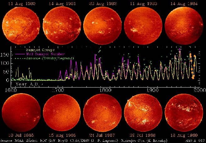
A touch of history
 • Self-exciting fluid dynamos are now a century-old idea
 • First invoked by Larmor in 1919 (sunspot magnetism)

 • The idea took a lot of time to gain ground
 • Cowling’s antidynamo theorem (1933)
 • First examples in the 1950s (e.g. Herzenberg dynamo)
 • Parker’s solar dynamo phenomenology (1955)

 • Golden age of mathematical theory
 • Alpha effect / mean-field: Steenbeck, Krause, Raedler 1966, Moffatt, Roberts etc. (1970s)
 • Small-scale dynamo theory: Kazantsev 1967, Kraichnan, Zel’dovich et al. (70s-80s)

 • Numerical and experimental era
 • Numerical evidence of turbulent dynamos: Meneguzzi et al. 1981, flourishing since then
 • Experimental evidence: Riga, Karlsruhe (~2000), VKS (2007), plasma underway (2005+)
 • Great observational radio and spectro-polarimetric prospects too (stellar, galactic, cosmo)

5 Astroplasma, March 2021
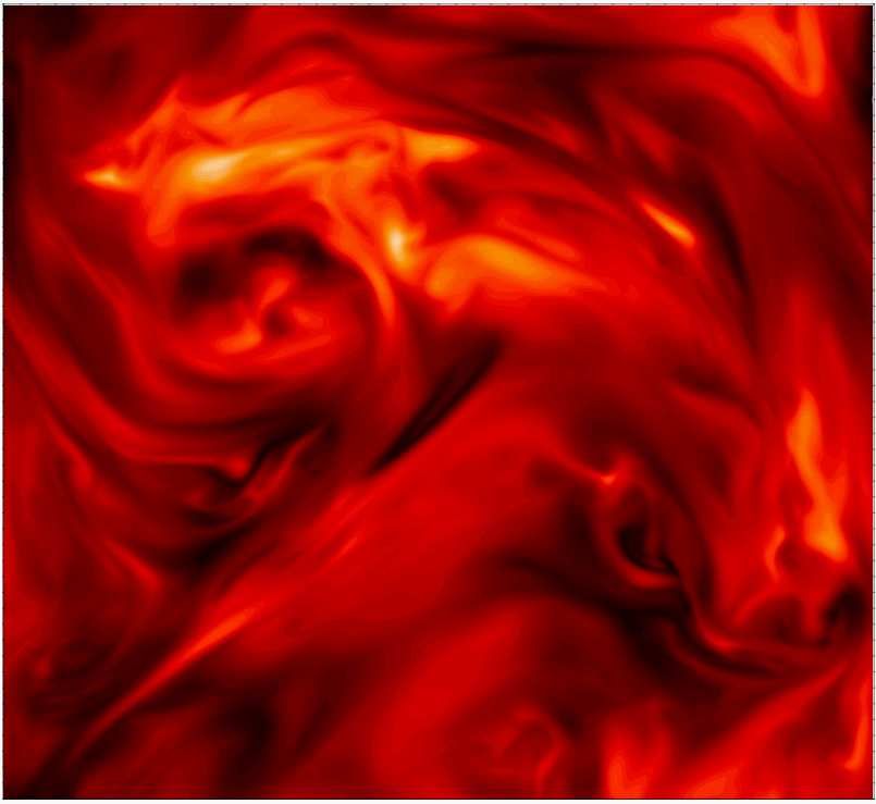
Solar magnetism
[Credits: SOHO/NASA]

 Global solar cycle dynamics
 ~ 1G-a few kG (sunspots)

 Small-scale surface dynamics
 ~ up to kG
6 [Credits: Hinode/JAXA] Astroplasma, March 2021
Planetary magnetism

[Swarm/ESA] [HST/NASA]

 Earth’s magnetic field (2014) ~ a few G Jupiter Auroras

7 Astroplasma, March 2021
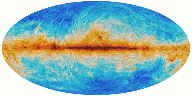
Galactic magnetism

 [Planck/ESA]

 Galactic magnetic field ~ 10 μG

 M51 magnetic field

 [Beck et al. VLA/Effelsberg]
8 Astroplasma, March 2021
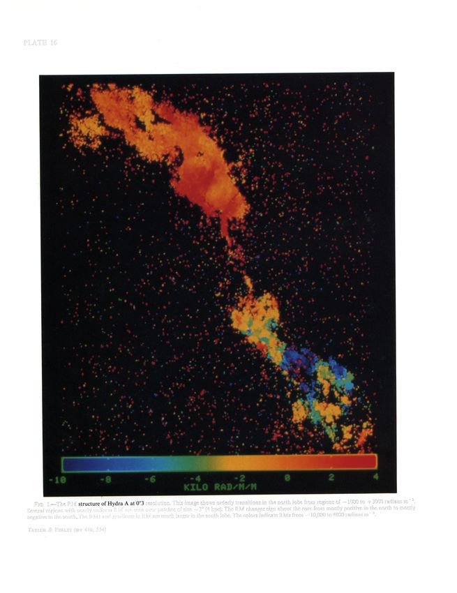
1993ApJ...416..554T
 Galaxy clusters and cosmic magnetism
 [Taylor & Perley, ApJ 1993]
[Fabian et al. ESA/NASA]
 Hydra A Lobe
Perseus/NGC 1275 filaments
 (25 kpc)

 ICM fields ~10 μG

 [Durrer & Neronov, A&A Rev. 2013]

 Clusters
 Galaxies

 Primordial
 IGMF limits

9
Takeaway phenomenological points
 • Many astrophysical objects have global, ordered fields
 • Differential rotation, global symmetries and geometry important
 • Coherent structures and MHD instabilities may also be very important
 • Motivation for the development of “large-scale” dynamo theories

 • Lots of “small-scale”, random fields also discovered from the 70s
 • These come hand in hand with global magnetism
 • Simultaneous development of “small-scale dynamo” theory

 • Astrophysical magnetism is in a nonlinear, saturated state
 • Linear theory likely not the whole story (or requires non-trivial justification)
 • Multiple scale interactions expected to be important

10 Astroplasma, March 2021
Setting the stage
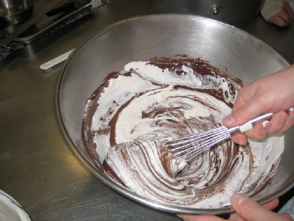
Mathematical formulation • Compressible, viscous, resistive MHD equations @⇢ + r · (⇢u) = 0 @t External forcing (spoon, Lorentz force ✓ ◆ gravity etc.) @u j⇥B ⇢ + u · ru = rp + + r · ⌧ + F(x, t) @t c Viscous stresses ✓ ◆ @ui @uj 2 Electromotive force ⌧ ij = µ + ij r ·u @B @xj @xi 3 = r⇥(u ⇥ B) r⇥(⌘r⇥B) @t Magnetic diffusion ⌘ = c2 4⇡ c r·B=0 j= r⇥B 4⇡ ✓ ◆ Dissipation Thermal diffusion @s ⇢T + u · rs = Dµ + D⌘ + r · (rT ) @t 12 Astroplasma, March 2021
Magnetic field energetics
 • Magnetic energy equation

 Z 2 Z I Z
 d B (j ⇥ B) c j2
 dV = u· dV (E ⇥ B) · dS dV
 dt 8⇡ c 4⇡
 Minus the work of the
 Poynting flux Ohmic dissipation
 Lorentz force on the flow

 • Magnetic field is generated at the expense of kinetic energy

 • Simple but enlightening local equation (ideal MHD)

 1 DB
 = b̂b̂ : ru r·u
 B Dt B
 Stretching Compression b̂ =
 D @ rate rate
 B
 = +u·r
 Dt @t
13 Astroplasma, March 2021
Conservation laws in ideal MHD
 • Alfvén’s theorem(s)
 • Magnetic field lines are “frozen into” the fluid just as material lines
 ✓ ◆
 D B B D r
 = · ru = r · ru
 Dt ⇢ ⇢ Dt
 • Magnetic flux through material surfaces is conserved
 D
 (B · S) = 0 S
 Dt
 Z
 • Magnetic helicity Hm = A · B d3 r conservation
 • A measure of magnetic linkage / knottedness
 1 @A
 = E r'
 c @t
 @
 (A · B) + r · [c'B + A ⇥ (u ⇥ B)] = 0
 @t
14 Astroplasma, March 2021
Simple MHD system for dynamo theory
 • Incompressible, resistive, viscous MHD
 • Captures a great deal of the dynamo problem
 Magnetic tension
 @u
 + u · ru = rP + B · rB + ⌫ u + f (x, t)
 @t
 Induction/stretching B2
 @B P =p+
 + u · rB = B · ru + ⌘ B 2
 @t Advection Resistive diffusion

 r·u=0 r·B=0 p and B rescaled by ⇢ and (4⇡⇢)1/2

 • Often paired with simple periodic boundary conditions
 • Can be problematic in some cases (more later)

15 Astroplasma, March 2021
Scales and dimensionless numbers
 • System/integral scale ℓ0, U0
 • Fluid system with two dissipation channels
 • Dimensionless numbers:
 `0 U0 `0 U0 ⌫
 Re = Rm = Pm =
 ⌫ ⌘ ⌘

 • Kolmogorov viscous scale ℓν ~ Re-3/4 ℓ0 , uν ~ Re-1/4 U0
 • Magnetic resistive scale ℓη (Pm-dependent)

 • Another important dimensionless quantity
 • Eddy turnover time NL ~ ℓu/u ⌧c
 St = Strouhal/Kubo number
 • Flow/eddy correlation time c ⌧NL

16 Astroplasma, March 2021
The magnetic Prandtl number landscape
 • Wide range of Pm in nature ⌫
 Liquid metals have Pm 1 makes Plasma exp.
 Liquid metals exp.
 life easier for magnetic fields Re
 1 104 108 1012

17 Astroplasma, March 2021
Large magnetic Prandtl numbers
 • Pm > 1: resistive cut-off scale is smaller than viscous scale
 • In Kolmogorov turbulence, rate of strain goes as ℓ-2/3

 • Viscous eddies are the fastest at stretching B: uν / ℓν ~ Re1/2 U0 / ℓ0
 • To estimate the resistive scale ℓη, balance stretching by these
 eddies ~ uν/ℓν with ohmic diffusion rate η/ℓη2

 1/2
 `⌘ ⇠ Pm `⌫
 e.g. galaxies, clusters
 Spectral power

 k-5/3
 forcing
 scales Magnetic energy
 spectrum tail
 Kinetic energy
 spectrum

 Wavenumber
 k
 k0 kν ∼ Re3/4 k0 kη ∼ Pm1/2kν >> kν

18 Astroplasma, March 2021
Low magnetic Prandtl numbers
 • Pm < 1: resistive cut-off falls in the turbulent inertial range
 • To estimate the resistive scale ℓη, balance magnetic stretching by the
 eddies at the same scale ~ uη/ℓη, with diffusion η/ℓη2

 • i.e., Rm (ℓη) = u(ℓη) ℓη / η ~ 1

 3/4
 `⌘ ⇠ Pm `⌫ e.g. stellar, solar,
 liquid metals (Earth, experiments)

 k-5/3 Kinetic energy
 Spectral power

 forcing spectrum
 scales
 Magnetic energy
 spectrum tail

 Wavenumber
 k
 k0 kη ∼ Pm3/4 kν
Dynamo fundamentals
 • The problem of exciting a dynamo is an instability problem
 `0 U0
 • Growth requires stretching to overcome diffusion (measured by Rm = )
 ⌘
 @B
 • Kinematic dynamo problem: + u · rB = B · ru + ⌘ B
 @t
 • Find exponentially growing solutions of the linear induction equation

 (velocity field is prescribed)

 • Dynamical problem considers effects of Lorentz force on u
 • Saturated state of kinematic dynamos: non-linear magnetic back reaction
 • Subcritical scenarios: e.g. joint excitation of u and B via MHD instabilities

 • Slow vs Fast
 • A dynamo is slow/fast if its growth rate does/doesn’t vanish as ⌘ ! 0

20 Astroplasma, March 2021
Cowling’s antidynamo theorem
 • Axisymmetric dynamo action is impossible [Cowling, MNRAS, 1933]
 ez
 • In polar geometry, write e'
 Poloidal Toroidal z er
 • B = r ⇥ ( e' /r) + r e'
 • u = upol + r⌦ e' ' r
 ✓ ◆
 @ 2 @
 + upol · r = ⌘ No source term
 @t r @r
 ✓ ◆
 @ 2 @
 + upol · r = Bpol · r⌦ + ⌘ +
 @t r @r
 • Poloidal flow can only redistribute flux so must decay ultimately
 • As decays, so must the toroidal field

 • Note: only applies if u and B share the same symmetry axis

21 Astroplasma, March 2021
Antidynamo theorems and their implications
 • Many other antidynamo results can be proven
 • Plane two-dimensional motions cannot sustain a dynamo
 [Zel’dovich’s theorem, JETP 1957]

 • A purely toroidal flow cannot sustain a dynamo
 • B(x, y, t) cannot be a dynamo field

 • Dynamos are only possible in “complex” geometries or flows
 • An extra burden for both theory and numerics
 • A popular “minimal” configuration is 2.5D (or 2D-3C)
 • u(x, y, t) with all three components non-vanishing
 • B(x, y, z, t) = R b(x, y, t)eikz z

22 Astroplasma, March 2021
The fast dynamo paradigm
 [Vainshtein & Zel’dovich, SPU, 1972]

 • Chaotic stretching, twisting, folding and merging of field lines
 • For small diffusion, field doubles at each “iteration” (characteristic time)
 • Exponential growth with “ideal” growth rate 1 = ln 2 ~ stretching rate

 Stretch

 Twist

 3D essential ! Lyapunov exponents of
 Galloway-Proctor flow
 [credits F. Cattaneo]

 Merge
 (requires a tiny bit
 of magnetic diffusion !)
 [adapted from Brandenburg &
 Fold
 Subramanian, Phys. Rep. 2005]

23 Astroplasma, March 2021
MHD dynamos
 II. Textbook theory & numerics

 François Rincon

 Bed time reading:

 Dynamo theories
 J. Plasma Phys. (Lecture Notes Series) 85, 205850401 (2019)
 arXiv:1903.07829
Les Houches, May 2017
An imperfect dichotomy
 • Large-scale dynamo effect
 • Magnetic field generated on

 • long system time (Ω−1, S −1), spatial scales (L) much larger than flow scales ℓ0

 • also lots of magnetic fluctuations on low and sub flow scales down to the magnetic resistive scale

 • Small-scale dynamo effect
 • Magnetic field generated on short time (ℓ/u), spatial scales (ℓ) from flow scales down to the resistive scale

 • Each of these can be excited by laminar or turbulent flows

 • They have traditionally mostly been described by different theories
 • in all MHD astrophysical settings, large-scale dynamos are swamped by small-scale ones
 • this creates a lot of theoretical difficulties

 • MHD instabilities also play a key role in large-scale dynamos
 • the magneto-rotational, and other magnetoshear instabilities
 • Kelvin-Helmholtz instability coupled to magnetic buoyancy

25 Astroplasma, March 2021
Large vs small magnetic Prandtl numbers

 k-5/3 Kinetic energy e.g. stellar, solar,
 Spectral power

 forcing spectrum liquid metals (Earth, experiments)
 scales
 Magnetic energy 3/4
 spectrum tail `⌘ ⇠ Pm `⌫

 Wavenumber
 k
 k0 kη ∼ Pm3/4 kν > kν

26 Astroplasma, March 2021
Small-scale dynamo theory
how to make magnetic fields on scales
 comparable to flows
Numerical evidence
 • Homogeneous, isotropic, non-helical, incompressible, 3D
 turbulent flow of conducting fluid is a small-scale dynamo

 64x64x64 spectral direct numerical simulations at Pm=1

 [Meneguzzi, Frisch, Pouquet, PRL, 1981]

28 Astroplasma, March 2021
Zel’dovich-Moffatt-Saffman phenomenology
 [Moffatt & Saffman, 7, 155 (1964); Phys. Fluids, Zel’dovich et al., JFM 144, 1 (1984)]

 • Consider incompressible, kinematic dynamo problem
 @B
 + u · rB = B · ru + ⌘ B r·B=0
 @t
 • Assume that B(0, r) = B0 (r)
 • has finite total, energy, no singularity
 • lim B0 (r) = 0
 r!1

 • Take simplest possible model of time-evolving “smooth” velocity field

 • Random linear shear: u = Cr Tr C = 0 [incompressible]

 [think of this as being 3D]
29 Astroplasma, March 2021
Stretching and squeezing
 d ri
 • Evolution of vector connecting 2 fluid particles: = Cik rk
 dt
 • Consider constant C = diag(c1 , c2 , c3 )
 c1 + c2 + c3 = 0
 • Exponential stretching along first axis
 c 1 > 0 > c2 > c3 c 1 > c2 > 0 > c3
 e1 e2 e1
 e2 e3
 e3

 “rope”
 “pancake”

 • In ideal MHD, we thus expect B 2 ⇠ exp(2c1 t)
 • However, perpendicular squeezing implies that even a tiny magnetic
 diffusion matters…is growth still possible in that case ?
30 Astroplasma, March 2021
Magnetic field evolution
 Z
 • Decompose B(t, r) = b(t, k0 ) exp (ik(t) · r)d3 k0
 db 2dk
 = Cb ⌘k b = CT k k·b=0
 dt dt ✓ Z
 t ◆
 • Diffusive part of evolution ~ exp ⌘ k 2 (s)ds
 0
 • super-exponential decay of most Fourier modes because

 k3 ⇠ k03 exp(|c3 |t)

 • surviving modes live in an exponentially narrow k-cone such that
 Z t
 ⌘ k 2 (s)ds = O(1)
 0

 • rope case: k02 ⇠ exp( |c2 |t) k03 ⇠ exp( |c3 |t)

31 Astroplasma, March 2021
Magnetic field evolution (ropes)
 • Surviving modes at time t have an initial field e1

 • b1 (0, k0 ) ⇠ b2 (0, k0 )k02 /k01 ⇠ exp( |c2 |t) e2
 e3

 • This field is stretched along the first axis, so

 b(t, k0 ) ⇠ exp (c1 t) exp ( |c2 |t)

 • Now, estimate the magnetic field in physical space
 Z
 B(t, r) ⇠ Bk d3 k0 ⇠ exp( |c2 |t)

 ⇠ exp [(c1 |c2 |)t] ⇠ exp [( |c2 | |c3 |)t]

 Magnetic field stretches into an asymptotically-decaying rope
32 Astroplasma, March 2021
Magnetic energy evolution (ropes)
 • What about magnetic energy ? e1

 Z e2
 e3
 2 3
 Em = B (t, r)d r

 Volume ⇠ exp(c1 t)
 B 2 ⇠ exp ( 2|c2 |t) Important: no shrinking along axis 2 and 3 as
 diffusion sets a minimum scale in these directions

 Em ⇠ exp [(c1 2|c2 |)t] ⇠ exp [(|c3 | |c2 |)t] (3D)

 Total magnetic energy grows ! (in 3D)

 Volume occupied by the magnetic field grows faster than field decays pointwise

 • Similar conclusions apply in the pancake case, but Em ⇠ exp [(c1 c2 )t]

33 Astroplasma, March 2021
Generalization to random, time-dependent shear • Renovate shear flow every time-interval • Succession of random area-preserving stretches and squeezes • Introduce the matrix Tt ⌘ T(t0 , t) such that k(t, k0 ) = Tt k0 Y t ⇥ ⇤ • Volterra multiplicative integral form: Tt = CT (s)ds s=0 Product of unimodular • Formal solution random matrices Z Z t B(t, r) = exp iTt (k0 · r) ⌘ (Ts k0 )2 ds (TTt ) 1 b(0, k0 )d3 k0 0 • Hard work: calculate the properties of the multiplicative integral ! 34 Astroplasma, March 2021
Lyapunov basis of random shear flow
 • Zel’dovich showed that the cumulative effects of any random
 sequence of shears can be reduced to diagonal form
 • In particular there is always a net positive “stretching” Lyapunov exponent

 1
 lim ln k(n⌧, k0 ) ⌘ 1 >0
 n!1 n⌧

 • The underlying Lyapunov basis (e1 , e2 , e3 )
 • is a function of the full random sequence, but is independent of time
 • “cristallizes” exponentially fast in time (exponents converge as 1/t)

 • The problem reduces to that described earlier
 • Magnetic energy growth is possible in a smooth, 3D chaotic velocity field
 in the presence of magnetic diffusion

35 Astroplasma, March 2021
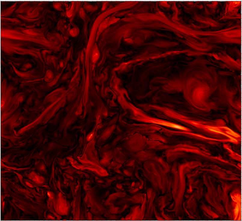
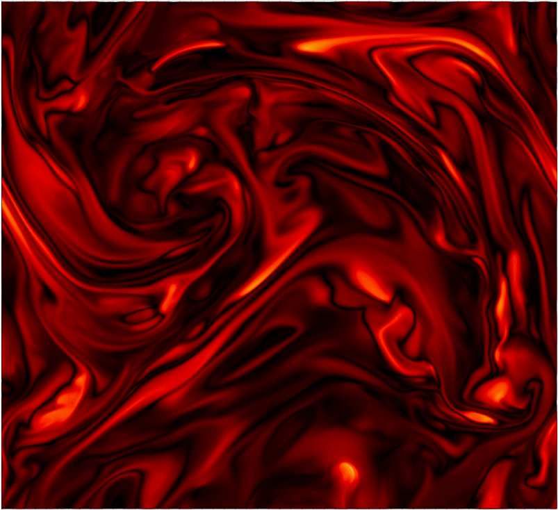
Small-scale dynamo fields at Pm ≥ 1
 • Pm=Rm=1250, Re=1 [from Schekochihin et al., ApJ 2004]
 u

 B

 • Folded field structure
 • Reversals at resistive scale 1/2
 `⌘ ⇠ `⌫ Pm
 • Folds coherent over flow scale
 Critical Rm ~ 60
 • Field strength and curvature anticorrelated
36 Astroplasma, March 2021
Small-scale dynamo at low Pm
 • Yes, but much harder Pm=1250, Re=1, Rm=1250

 • Critical Rm~200
 • More complicated than
 Pm=1, Re=440, Rm=440
 Zel’dovich picture

 Pm=0.07, Re=6200, Rm=430

 [Iskakov et al., PRL 2007]
37 Astroplasma, March 2021
Kazantsev-Kraichnan theory • Consider again the following kinematic dynamo problem: @B + u · rB = B · ru + ⌘ B r·B=0 @t • This problem can be solved analytically if u is • a random Gaussian process with no memory (zero-correlation time) • The so-called Kraichnan ensemble ⌦ 0 0 ↵ u (x, t)u (x , t ) = ij (r) (t i j t0 ) • Obviously, not your usual turbulent flow, but still… • Very useful to understand some properties of small-scale dynamo modes • Originally solved by Kazantsev [JETP, 1968] [and further explored by Zel’dovich, Ruzmaikin, Sokoloff, Vainshtein, Kitchatinov, Vergassola, Vincenzi, Subramanian, Boldyrev, Schekochihin etc.] 38 Astroplasma, March 2021
Equation for magnetic correlations
 • Goal: derive a closed equation for the two-point, single time
 magnetic correlator [or magnetic energy spectrum]
 ⌦
 B i (x, t)B j (x0 , t) = H ij (x x0 , t)
 ✓ i j
 ◆ i j
 0 r r r r
 H ij (x x , t) = HN (r, t) ij
 2
 + HL (r, t) 2
 r r
 HN = HL + (rHL0 )/2

 • Induction equation at (x,t) and (x’,t) gives
 @H ij @ ⌦ i k 0 j 0
 ↵ ⌦ i j 0 k 0
 ↵
 = 0k
 B (x, t)B (x , t)u (x , t) B (x, t)B (x , t)u (x , t)
 @t @x Third order
 Second order @ ⌦ k j 0 i
 ↵ ⌦ i j 0 k
 ↵ moments
 + B (x, t)B (x , t)u (x, t) B (x, t)B (x , t)u (x, t)
 moment @x k
 ✓ ◆
 @ @ ij
 + ⌘ + H
 @xk @x0k
 @ @ @ [statistical
 h·i = h·i = h·i
 @x0k @xk @rk homogeneity]

39 Astroplasma, March 2021
The closed equation • Using properties of the Kraichnan ensemble, the problem reduces to a closed equation for magnetic correlator HL (r, t) ✓ ◆ ✓ ◆ @HL 4 4 0 = HL00 + 0 0 00 + H L + + HL @t r r (r) = 2⌘ + L (0) L (r) “Turbulent diffusivity” (twice) • Schrödinger equation with imaginary time 2 1/2 • Change variables: HL (r, t) = (r, t)r (r) @ 00 = (r) V (r) @t 1 • Wave function of quantum particle of variable m(r) = in potential 2(r) 2 1 00 2 0 0 (r)2 V (r) = 2 (r) (r) (r) r 2 r 4(r) 40 Astroplasma, March 2021
Solutions 00 1 @ m(r) = [2(r)] = V (r) @t 2m(r) (r) = 2⌘ + L (0) L (r) 2 1 00 2 0 0 (r)2 V (r) = 2 (r) (r) (r) r 2 r 4(r) Et • Look for solutions of the form = E (r)e • Growing dynamo modes correspond to discrete bound states: E> 1 and Pm
Different regimes ⌦ 00 00 ↵ • Recall u (x, t)u (x , t ) = i` (x i ` x00 ) (t t00 ) • So (r) ⇠ u(r)2 ⌧ (r) ⇠ r u(r) is a turbulent diffusivity • Consider the scaling law L (0) L (r) ⇠ r⇠ Roughness exponent • Smooth flow: u ⇠ r ) ⇠=2 [“large Pm”] • “Kolmogorov” turbulence: u ⇠ r1/3 ) ⇠ = 1 + 1/3 = 4/3 [“low Pm”] • Potential as a function of ⇠ Ve↵ (r) • Ve↵ (r) = 2/r2 , r ⌧ `⌘ p ⇠ < ⇠c = 11/3 1 3 3 2 2 `⌘ • Ve↵ (r) = (2 ⇠ ⇠ )/r , r `⌘ r 2 4 ⇠ > ⇠c • Growing bound modes for ⇠ > 1 • includes both Pm >> 1 and Pm
A few important results at large Pm • Consider the so called Batchelor regime `⌘ ⌧ `⌫ • The magnetic field is stretched and transported by a viscous flow 2 ✓ i j ◆ ij ij r ij 1r r • The velocity field is smooth: (r) = 0 2 2 + ··· 2 2 r • Spectral view at scales much smaller than the viscous scale • Work under Kazantsev-Kraichnan assumptions • Fokker-Planck type equation for the magnetic spectrum M(k) ✓ 2 ◆ @M 2@M @M = k 2 + 6M 2⌘k 2 M @t 5 @k 2 @k • Typical growth rate of the order of the shearing rate at viscous scales 5 5 [Kazantsev JETP 1968; = 2 = |00L (0)| ⇠ u⌫ /`⌫ 4 2 Kulsrud and Anderson, ApJ 1992; Schekochihin et al., ApJ 2002] 43 Astroplasma, March 2021
Large Pm, diffusion-free regime • Magnetic diffusion negligible if magnetic field only has k ⌧ k⌘ • If we excite a given k0 initially, the spectrum spreads towards small-scales ✓ ◆3/2 r k 5 5 ln2 (k/k0 ) M (k, t) / e3/4 t exp k0 4⇡ t 4 t • The energy of each mode grows at rate 3 /4 • Total energy grows at rate 2 as the number of excited mode also grows • The magnetic field develops the so-called k 3/2 Kazantsev spectrum M (k) E(k) k 3/2 Stirring k k⌫ k⌘ 44 Astroplasma, March 2021
Large Pm, resistive regime
 • After the spectrums hits k ⇠ k⌘ , the long-time asymptotics is
 ✓ ◆
 3/2 k 3/4 t
 p
 M (k, t) / k K0 e k⌘ = /(10⌘) ⇠ Pm1/2 k⌫
 k⌘

 • The spectrum peaks at the resistive scale [falls off exponentially beyond]
 • The asymptotic total energy growth rate is now also approximately 3 /4
 [weak dependence on boundary condition at small k]

 k 3/2 M (k)
 E(k)

 Stirring

 k
 k⌫ k⌘
45 Astroplasma, March 2021
Magnetic pdf in the diffusion-free regime • One can derive a Fokker-Planck equation for the pdf of B @ 2 ij k @ ` @ P [B] = Tk` B i B j P [B] @t 2 @B @B • Simplifies in the isotropic case as 1D diffusion equation with drift @ 2 1 @ 4 @ Z 1 pdf defined as P [B] = 2 B P [B] @t 4 B @B @B hB n (t)i = 4⇡ dBB 2+n P [B] 0 • Lognormal solution Z ! 1 2 1 dB 0 0 [ln(B/B 0 ) + (3/4)2 t] P [B](t) = p 0 P 0 [B ] exp ⇡2 t 0 B 2 t • The magnetic field is strongly intermittent / non-Gaussian 1 n • Magnetic moments grow as hB (t)i / exp n(n + 3)2 t 4 46 Astroplasma, March 2021
Saturation of small-scale dynamo
 • As B gets large-enough, Lorentz force saturates dynamo
 [Meneguzzi et al., PRL 1981]
 • What is “large-enough “?
 • How does it work ?

 • Historical ideas
 • Batchelor argument [PRSL,1950]:
 • magnetic field is similar to hydrodynamic vorticity
 • should peak at viscous scale, hence saturation for B 2 ⇠ u2⌫
 ⌦ 2↵ 1/2
 ⌦ 2↵
 B ⇠ Re u Sub-equipartition unless Re=1

 • Schlüter-Biermann argument [Z. Naturforsch.,1950]:
 ⌦ 2
 ↵ ⌦ 2
 ↵
 • equipartition at all scales B ⇠ u

47 Astroplasma, March 2021
Saturation phenomenology
 • Geometric structure and orientation of the field matters
 • Magnetic tension B · rB encodes magnetic curvature
 • Reduction of stretching Lyapunov exponents
 • A field realization can only saturate itself

 Kinematic Saturated Saturated magnetic field

 i c field
 et
 magn
 um my
 D

 [Cattaneo et al., PRL 1996] [Cattaneo & Tobias, JFM 2009]

 • Saturation at low Pm
 • Pretty much Terra incognita (almost no published simulation)

48 Astroplasma, March 2021
Large Pm phenomenology
 • Plausible (but not definitive) scenario from simulations
 [Schekochihin et al., ApJ 2002, 2004]

 • Lorentz force first suppresses stretching at viscous scales

 B · rB ⇠ u · ru ⇠ u2⌫ /`⌫ ⌦ ↵ 1/2
 ⌦ ↵
 2 2
 2
 B ⇠ Re u
 ⇠ B /`⌫ (folded structure)

 • From there, slower, larger-scale eddies take over stretching

 • B keeps growing and acts on increasingly more energetic eddies…
 ⌦ 2↵
 • Secular growth regime: B ⇠ "t
 ⌦ 2
 ↵ ⌦ 2
 ↵
 • Final state: B ⇠ u after “suppression” of full inertial range
 • “Isotropic MHD turbulence”, folded structure is preserved

 • P[B] not log-normal anymore (likely exponential)
49 Astroplasma, March 2021
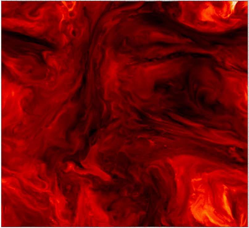
But…what about reconnection ?
 • New challenges…
 (a)
 (a) (b)(b)
 Dynamotheories
 Dynamo theories 4545
 Courtesy from Iskakov & Schekochihin (unpublished)

 (c)
 (c) (d)(d)
 Figure
 Figure23.23.2D |u|
 snapshotsofof|u|
 2Dsnapshots |u|(left) and|B|
 (left)and |B|(right)
 (right)inina anonlinear |B|
 nonlinearsimulation
 simulationof ofsmall-scale
 small-scale
 dynamo
 dynamodriven
 drivenbybyturbulence
 turbulenceforced
 forcedatatthe theboxboxscale
 scaleatatReRe==290 290Rm Rm=Re=290, 2900,P Rm=2900,
 =2900, P m= =1010 Pm=10
 m
 3 3
 (the
 (themagnetic
 magneticenergy
 energyspectra
 spectrafor
 forthis
 this512
 512 spectral
 spectralsimulation
 simulationsuggest
 suggestthat
 thatit it
 is is
 reasonably
 reasonably well
 well
 • More
 resolved).
 resolved). in
 AtAtsuch
 suchmy
 largefinal
 large Rm,seminar
 Rm, the
 thedynamo next
 dynamo fiedtime…
 fiedbecomes
 becomesweaklyweaklysupercritical
 supercriticaltotoa asecondary
 secondary
 fast-reconnection
 fast-reconnectioninstability
 instabilityininregions
 regionsofofreversing
 reversingfield
 fieldpolarities
 polaritiesassociated
 associatedwith withstrong
 strong
50 electrical
 electricalcurrents.
 currents.TheTheinstability
 instabilitygenerates
 generatesmagnetic
 magneticplasmoids
 plasmoidsandandoutflows, Astroplasma,
 leavinga a March 2021
 outflows,leaving
Large-scale dynamo theory
how to build-up magnetic fields on system
 scales much larger than flow scales
Differential rotation: the Omega effect
 • Shearing of magnetic field by differential rotation (shear)
 • In polar geometry, consider the initial axisymmetric configuration
 • a purely poloidal magnetic field: Bpol = Br (r, z)er + Bz (r, z)ez
 • a toroidal, shearing velocity field (differential rotation): u = r⌦(r, z)e'
 ✓ ◆
 @B' 1
 = r(Bpol · r)⌦ + ⌘ B'
 @t r2
 • On short times, B' can grow linearly in time
 • Ultimately, diffusion always dominates

 • This effect alone cannot produce a dynamo (Cowling)
 • But it can transiently make strong toroidal field out of weak poloidal field

52 Astroplasma, March 2021
Turbulence: Parker’s mechanism
 • Effect of a localized cyclonic swirl on a straight magnetic field

 [Parker, ApJ 1955] [Moffatt, Les Houches lectures 1973]

 • In polar geometry, this mechanism can produce axisymmetric poloidal field out
 of axisymmetric toroidal field — and the converse
 • Kinetic helicity in the swirl is essential

 • This “alpha effect” can mediate statistical dynamo action
 • Ensemble of turbulent helical swirls should have a net effect of this kind
 • Cowling’s theorem does not apply as each swirl is localized (“non-axisymmetric”)

53 Astroplasma, March 2021
Numerical evidence
 • Small-scale helical turbulence can generate large-scale field
 • Critical Rm is O(1), lower than that of the small-scale dynamo
 [Brandenburg, ApJ 2001]
 [Meneguzzi et al., PRL 1981 — again !]

 • Helicity seemingly key for large-scale dynamos (but see later)
54 Astroplasma, March 2021
Twisting and magnetic helicity
 • Assume conservation of magnetic helicity (up to resistive effects)
 • Systematic twisting produces
 • negative large-scale magnetic helicity (large-scale writhe)
 • positive small-scale magnetic helicity (small-scale twist)

 [adapted from Mininni, ARFM 2011]

 • Consequences
 • Interpretation of large-scale helical dynamo as “inverse transfer” of helicity
 [Frisch et al., JFM 1975]
 • Transfer of helicity at small scales

55 Astroplasma, March 2021
Mean-field approach
 • Incompressible, kinematic problem with uniform diffusivity
 @B
 = r⇥(u ⇥ B) + ⌘ B
 @t

 r·u=0 r·B=0

 • Split fields into large-scale (` > `0 ) and fluctuating part (` < `0 )

 B = B + B̃ u = u + ũ

 @B ⇣ ⌘
 + u · rB = B · ru + r ⇥ ũ ⇥ B̃ + ⌘ B
 @t

 • To determine the evolution of B we need to know E = ũ ⇥ B̃
 • We cannot just sweep fluctuations under the rug: closure problem

56 Astroplasma, March 2021
Mean-field approach
 @ B̃ h ⇣ ⌘ ⇣ ⌘ ⇣ ⌘i
 = r ⇥ ũ ⇥ B + u ⇥ B̃ + ũ ⇥ B̃ ũ ⇥ B̃ + ⌘ B̃
 @t
 Tangling/shearing Tricky bit — closure problem !
 of mean field [also known as the “pain in the neck” term]

 • Assume linear relation between B̃ and B [Warning: hard to justify if
 there is small-scale dynamo !]
 • Expand (ũ ⇥ B̃)i = ↵ij Bj + ijk rk Bj + · · ·
 • Simplest pseudo-isotropic case: ↵ij = ↵ ij, ijk = ✏ijk

 • For u = 0 , we obtain a closed “↵2“ dynamo equation (⌘ ⌧ )
 @B
 = r ⇥ ↵B + B
 @t
 alpha effect beta effect (“turbulent” diffusion)

 • Exponentially growing solutions with real eigenvalues = |↵|k k2
 • Max growth rate max = ↵2 /(4 ) at scale `max = 2 /↵ `0
57 Astroplasma, March 2021
Mean-field dynamo with Omega effect
 • Add large-scale differential rotation to MF equation: u = r⌦(r, z)e'
 @B
 = e' r (Bpol · r) ⌦ + r ⇥ ↵B + B
 @t
 Omega effect Alpha effect

 • Growing, oscillatory solutions leading to field reversals: Parker waves
 2
 • This is called the ↵⌦ dynamo ( ⌦ if ↵ acts both ways)
 ↵

 ⌦ effect (+↵ effect)

 Poloidal field Toroidal field

 ↵ effect
 • Remarks
 • Many other couplings possible: pumping effects, non-diagonal terms etc.
 • 3Dness of the dynamo is hidden in mean-field coefficients

58 Astroplasma, March 2021
Calculation of mean-field coefficients
 • We only know how to calculate ↵ and perturbatively for
 • small correlation times (low Strouhal number ⌧c /⌧NL, random waves)
 • low magnetic Reynolds number Rm ⇠ ⌧⌘ /⌧NL ⌧ 1

 @ B̃ h ⇣ ⌘ ⇣ ⌘i (u=0)
 ˙
 = r ⇥ ũ ⇥ B + ũ ⇥ B̃ ũ ⇥ B̃ + ⌘ B̃
 @t

 O(B̃rms /⌧c ) O(B/⌧NL ) O(B̃rms /⌧NL ) O(B̃rms /⌧⌘ )
 ⌧NL = `u /urms tricky “pain in the neck” term G ⌧⌘ = `2u /⌘

 • In both cases we can justify neglecting the tricky term
 • First Order Smoothing Approximation (FOSA, SOCA, Born, quasilinear…)

 [Steenbeck et al., Astr. Nach. 1966; see H. K. Moffatt’s textbook, CUP 1978;
 Brandenburg & Subramanian, Phys. Rep. 2005]

59 Astroplasma, March 2021
Calculation of mean-field coefficients
 • Let’s see how the calculation proceeds for ⌧c /⌧NL ⌧ 1
 • Neglecting the tricky term and assuming small resistivity,
 Z t ⇥ ⇤
 ũ(t) ⇥ B̃(t) = ũ(t) ⇥ r⇥ ũ(t0 ) ⇥ B(t0 ) dt0
 0
 Z th i
 = ˆ (t t0 )B(t0 )
 ↵ ˆ(t t0 )r ⇥ B dt0 (isotropic case)
 0
 1 0 ˆ 1
 ˆ = ũ(t) · !(t
 ↵ ˜ ) = ũ(t) · ũ(t0 ) ˜ = r ⇥ ũ
 !
 3 3
 • For slowly varying B and short-correlated velocities, this simplifies as

 ũ(t) ⇥ B̃(t) = ↵B r⇥B
 1 1
 ↵' ⌧c (ũ · !)
 ˜ ' ⌧c ũ2
 3 3
 • The role of kinetic helicity is explicit
 1
 • At low Rm, we have the similar result ↵ ' ⌧⌘ (ũ · !)
 ˜
 3
60 Astroplasma, March 2021
Dynamical regime of large-scale dynamos
 • When B gets “large enough”, the Lorentz force back-reacts
 • Big questions: what happens then, and what is “large-enough” ?
 [Brandenburg & Subramanian, Phys. Rep. 2005, and refs. therein: Proctor, 2003; Diamond et al. 2005]

 2 2
 • Equipartition argument: saturation when B ⇠ 4⇡⇢ ũ2 ⌘ Beq , but
 • B and ũ have very different scales
 • Large-scale dynamos alone produce plenty of small-scale field

 2
 • Equipartition of small-scale fields: b̃2 ⇠ 2
 Beq , with b̃2 ⇠ Rm Bp

 2
 • 2
 Not very astro-friendly: B ⇠ Beq /Rmp ⌧ Beq
 2
 for p=O(1)
 • Possibility of “catastrophic” alpha quenching
 ↵0
 ↵(B) =
 q
 2 )
 1 + Rm (B /Beq
 2 q = O(1)

61 Astroplasma, March 2021
The quenching issue
 • Physical origin of quenching debated:
 • Magnetized fluid has “memory”: possible drastic reduction of statistical effects
 compared to random walk estimates [see review by Diamond et al., 2005]

 • Magnetic helicity conservation argument:
 • in “closed” systems, large-scale field can only reach equipartition
 on slow, large-scale resistive timescales [e.g. Brandenburg, ApJ 2001]

 • Possible way out of problem is to ”evacuate” magnetic helicity
 [Blackman & Field, ApJ 2000; see discussion by Brandenburg, Space Sci. Rev. (2009)]
 78 F. Rincon
 d [Bhat et al., MNRAS 2016]
 hA · BiV = 2⌘ h (r(a)⇥ B) · BiV hr · FHm i (b)
 dt
 • Open boundary conditions (periodic b.c. not ok)
 • Internal fluxes of helicity [Kleeorin et al., Vishniac-Cho etc.]

 • More on this in my final seminar next time
62 F IGURE 31. (a) Magnetic (full black lines) and kinetic energy (dotted blueMarch
 Astroplasma, lines) 2021
 spectr
Large vs small-scale
 growth: who wins ?
Large-scale dynamos with Kasantsev [Vainshtein & Kitchatinov, JFM 1986, Berger & Rosner, GAFD 1995, • Consider turbulence with net helicity Subramanian, PRL 1999, Boldyrev et al., PRL 2005] • Add a mirror symmetry-breaking term to the correlators ✓ i j ◆ ij ij rr ri rj (r) = N (r) + L (r) 2 + g(r)"ijk rk r2 r ✓ i j ◆ rr ri rj H ij (x x0 , t) = HN (r, t) ij 2 + H L (r, t) 2 + K(r)" ijk k r r r 2 • r ! 1 asymptotics of model gives mean-field ↵ equation @B L (0) = r ⇥ ↵B + (⌘ + ) B g(0) = ↵, = @t 2 • Full calculation leads to coupled equations for HL and K ✓ ◆ @HL 1 @ @HL 4 = 4 r + GHL 4hK h(r) = g(0) g(r) @t r @r @r @K 1 @ 4 @ G(r) = 00 + 40 /r = 4 r (K + hHL ) @t r @r @r 64 Astroplasma, March 2021
Self-adjoint spinorial form @W p = R̃T J˜R̃W A(r) = p 2 [2⌘ + N (0) N (r)] @t B(r) = 2 [2⌘ + L (0) L (r)] p p ! ✓ ◆ C(r) = 2 [g(0) g(r)] r 2/r 0 Ê C 1 @ @ 1 R̃ = 1 @ 2 J̃ = Ê = r B r + p (A rA0 ) 0 r C B 2 @r @r 2 2 r @r 2 p p p 30 p 0 1 2 2 2 @ 2 1 2 WH Ê C(r) r WH HL = 2 W H @ @ A=6 r rp r3 @r 7@ A rp 4 5 @t 2 @ 2 2 @ B(r) @ 2 2 @ 2 WK r C(r) 3 r r WK K= 4 (r WK ) @r r 4 @r r @r r @r • Therefore, the generalized helical case can be diagonalized g 2 (0) 2↵2 • Bound “small-scale” modes: n > 0 0 = = L (0) + 2⌘ 4( + ⌘) • Free “mean-field” modes: 0 < < 0 Twice the maximum ↵ 2 mean-field dynamo growth rate ! 65 Astroplasma, March 2021
Growing helical modes
 • Helicity allows growing large-scale Ve↵ (r)

 modes
 2 2 2 `⌘
 • Ve↵ (r) = 2/r ↵ /( + ⌘) , `0 ⌧ r r
 `0

 • Bound modes ( > 0) dominate the [Malyshkin & Boldyrev, ApJ 2009]

 kinematic stage

 • As ! 0 , their spectrum peak shifts
 towards that of “mean-field” modes

 • Further hints that quantitative large-scale dynamo theory
 should factor in the small-scale dynamo
66 Astroplasma, March 2021
A few words on “test field”-like methods
 • Pragmatic strategies have been devised for “astrophysical applications”
 • postulate generalised mean-field form for E(B) (convolution integrals)
 • Measure effective transport coefficients in local simulations
 [Sur et al., MNRAS 2008,
 • Use the results in simpler 2D mean-field models Brandenburg, Space Sci. Rev. 2009]

 • Such procedures
 • produce converged values of transport coefficients
 • reproduce exact results in perturbative kinematic limits

 • TFM-based modelling may be useful, but:
 • no rigorous justification as to why it should be accurate/appropriate (Rm>>1 !)
 • dynamical, tensorial convolution relations E(B) can fit complex dynamics,
 but could well be degenerate with more physically-grounded nonlinear models
 • it can obfuscate the underlying physics, e.g. when MHD instabilities are involved

67 Astroplasma, March 2021
Situation so far
 • Historically, mean-field models have been at the core of modelling of
 • solar and stellar dynamos — “alpha” provided by cyclonic convection
 • galactic dynamos — “alpha” provided by supernova explosions

 • But classical mean-field theory faces strong limitations
 • Astro turbulence typically has ⌧c /⌧NL ⇠ 1 and Rm 1
 • “Co-existence” with fast, small-scale dynamo for Rm 1
 • pain in the neck term exponentially growing…then what ?
 • linear relation between b̃ and B doubtful
 • Non-linear quenching

 • Large-scale dynamos are “real” — independently of our limited theories
 • We have to think harder ! (and ask good questions to computers)
68 Astroplasma, March 2021
Tomorrow’s fundamental theory challenges
 • Turbulent large and small-scale MHD dynamos
 • Unified, self-consistent nonlinear multiscale statistical dynamo theory
 • Requires physically justified closures
 • Description of asymptotic regimes (very high Re and Rm, low Pm, strong rotation)

 • Interactions of different physical processes and geometrical effects
 • MHD instabilities combined to shear (magnetic buoyancy, MRI etc.)
 • Coherent structures (vortices, zonal flows, convection columns, tangent cylinders)
 • Reconnection in dynamos
 • Plasma effects (batteries, pressure anisotropies, partial ionization etc.)

 • History of cosmic magnetism
 • from the pre-CMB era to stellar and planetary magnetic fields

69 Astroplasma, March 2021
Today & tomorrow’s frontiers…next time !
 • Dynamos meet reconnection
 • Asymptotic nonlinear dynamos
 • Plasma (kinetic) dynamo

 Next presentation will be essentially equation-free
You can also read