Tropospheric Ozone Assessment Report: Tropospheric ozone from 1877 to 2016, observed levels, trends and uncertainties - University of ...
←
→
Page content transcription
If your browser does not render page correctly, please read the page content below
Tarasick, D, et al. 2019. Tropospheric Ozone Assessment Report: Tropospheric
ozone from 1877 to 2016, observed levels, trends and uncertainties. Elem Sci
Anth, 7: 39. DOI: https://doi.org/10.1525/elementa.376
REVIEW
Tropospheric Ozone Assessment Report: Tropospheric
ozone from 1877 to 2016, observed levels,
trends and uncertainties
David Tarasick*, Ian E. Galbally†,‡, Owen R. Cooper§,‖, Martin G. Schultz¶,
Gerard Ancellet**, Thierry Leblanc††, Timothy J. Wallington‡‡, Jerry Ziemke§§, Xiong Liu‖‖,
Downloaded from http://online.ucpress.edu/elementa/article-pdf/doi/10.1525/elementa.376/435292/376-6503-1-pb.pdf by guest on 05 January 2021
Martin Steinbacher¶¶, Johannes Staehelin***, Corinne Vigouroux†††, James W. Hannigan‡‡‡,
Omaira García§§§, Gilles Foret‖‖‖, Prodromos Zanis¶¶¶, Elizabeth Weatherhead§,‖,
Irina Petropavlovskikh§,‖, Helen Worden‡‡‡, Mohammed Osman****,††††,‡‡‡‡, Jane Liu§§§§,‖‖‖‖,
Kai-Lan Chang§,‖, Audrey Gaudel§,‖, Meiyun Lin¶¶¶¶,*****, Maria Granados-Muñoz†††††,
Anne M. Thompson§§, Samuel J. Oltmans‡‡‡‡‡, Juan Cuesta‖‖‖, Gaelle Dufour‖‖‖,
Valerie Thouret§§§§§, Birgit Hassler‖‖‖‖‖, Thomas Trickl¶¶¶¶¶ and Jessica L. Neu******
From the earliest observations of ozone in the lower atmosphere in the 19th century, both measurement
methods and the portion of the globe observed have evolved and changed. These methods have different
uncertainties and biases, and the data records differ with respect to coverage (space and time), information
content, and representativeness. In this study, various ozone measurement methods and ozone datasets
are reviewed and selected for inclusion in the historical record of background ozone levels, based on
relationship of the measurement technique to the modern UV absorption standard, absence of interfering
pollutants, representativeness of the well-mixed boundary layer and expert judgement of their credibility.
There are significant uncertainties with the 19th and early 20th-century measurements related to
interference of other gases. Spectroscopic methods applied before 1960 have likely underestimated ozone
by as much as 11% at the surface and by about 24% in the free troposphere, due to the use of differing
ozone absorption coefficients.
There is no unambiguous evidence in the measurement record back to 1896 that typical mid-latitude
background surface ozone values were below about 20 nmol mol–1, but there is robust evidence for increases
in the temperate and polar regions of the northern hemisphere of 30–70%, with large uncertainty, between
the period of historic observations, 1896–1975, and the modern period (1990–2014). Independent historical
observations from balloons and aircraft indicate similar changes in the free troposphere. Changes in the
southern hemisphere are much less. Regional representativeness of the available observations remains a
potential source of large errors, which are difficult to quantify.
The great majority of validation and intercomparison studies of free tropospheric ozone measurement
methods use ECC ozonesondes as reference. Compared to UV-absorption measurements they show a
modest (~1–5% ±5%) high bias in the troposphere, but no evidence of a change with time. Umkehr, lidar,
and FTIR methods all show modest low biases relative to ECCs, and so, using ECC sondes as a transfer
standard, all appear to agree to within one standard deviation with the modern UV-absorption standard.
Other sonde types show an increase of 5–20% in sensitivity to tropospheric ozone from 1970–1995.
Biases and standard deviations of satellite retrieval comparisons are often 2–3 times larger than those
of other free tropospheric measurements. The lack of information on temporal changes of bias for
satellite measurements of tropospheric ozone is an area of concern for long-term trend studies.
Keywords: Ozone; Troposphere; Measurements; Trends; Historical; Climate
Art. 39, page 2 of 72 Tarasick et al: Tropospheric Ozone Assessment Report
1. Introduction and 2) Generate easily accessible, documented data on
Tropospheric ozone is a greenhouse gas and pollutant ozone exposure metrics at thousands of measurement
detrimental to human health and plant growth (Monks sites around the world (Lefohn et al., 2018). Through the
et al., 2015; WMO Reactive Gases Bulletin, 2018). Large TOAR surface ozone database (Schultz et al., 2017; here-
changes after 1990 in the global distribution of the inafter TOAR-Surface Ozone Database) these ozone met-
anthropogenic emissions that produce ozone have been rics are freely accessible for research on the global-scale
reported, including reductions in North America and impact of ozone on climate (Gaudel et al., 2018), human
Europe and increases in Asia (Richter et al., 2005; Granier health (Fleming et al., 2018) and ecosystem productivity
et al., 2011; Russell et al., 2012; Hilboll et al., 2013; Cooper (Mills et al. 2018).
et al., 2014; Zhang et al., 2016). This rapid shift, coupled The assessment report is organized as a series of
with limited ozone monitoring in developing nations, has papers in a special feature of Elementa – Science of the
left scientists unable to answer the most basic questions: Anthropocene (https://collections.elementascience.org/
Which regions of the world have the greatest human and toar), with this paper comprising the Tropospheric Ozone
plant exposure to ozone pollution? How is ozone changing Assessment Report: Tropospheric ozone from 1877 to 2016,
Downloaded from http://online.ucpress.edu/elementa/article-pdf/doi/10.1525/elementa.376/435292/376-6503-1-pb.pdf by guest on 05 January 2021
in nations with strong emission controls? To what extent observed levels, trends and uncertainties, subsequently
is ozone increasing in the developing world? How can the abbreviated as TOAR-Observations. This paper describes
atmospheric sciences community facilitate access to the the different tropospheric ozone measurement tech-
ozone metrics necessary for quantifying ozone’s impact on niques used since the late 19th century to the present, and
climate, human health and crop/ecosystem productivity? characterizes the uncertainty in the measurements and
To answer these questions, the International Global the spatial and temporal information obtained from each
Atmospheric Chemistry Project (IGAC) developed the instrument type.
Tropospheric Ozone Assessment Report (TOAR): Global met- Knowledge of the uncertainties associated with tropo-
rics for climate change, human health and crop/ecosystem spheric ozone measurements is important to reconciling
research (www.igacproject.org/activities/TOAR). Initiated measurements from different methods and platforms and
in 2014, TOAR’s mission is to provide the research com- for accurate and realistic model evaluation. It is also essen-
munity with an up-to-date scientific assessment of tropo- tial for the evaluation of trends. Historical ozone observa-
spheric ozone’s global distribution and trends from the tions, those made before the widespread deployment of
surface to the tropopause. TOAR’s primary goals are, UV-based ozone instruments, are important to climate
1) Produce the first tropospheric ozone assessment report models. The global average radiative forcing of ozone
based on the peer-reviewed literature and new analyses, (0.4 ± 0.2 W m–2; IPCC, 2013) is approximately 1/5 of the
* Environment and Climate Change Canada, Downsview, ON, CA ¶¶¶
Department of Meteorology and Climatology, School of
†
Climate Science Centre, CSIRO Oceans and Atmosphere, Geology, Aristotle University of Thessaloniki, Thessaloniki,
Aspendale, VIC, AU GR
‡
Centre for Atmospheric Chemistry, University of Wollon-
****
Cooperative Institute for Mesoscale Meteorological Studies,
gong, Wollongong, NSW, AU The University of Oklahoma, US
§
Cooperative Institute for Research in Environmental
††††
NOAA/National Severe Storms Laboratory, Norman, OK, US
Sciences, University of Colorado, Boulder, US ‡‡‡‡
Enable Midstream Partners, Headquarters, Oklahoma City, US
‖
NOAA Earth System Research Laboratory, Boulder, Colorado, US §§§§
Department of Geography and Planning, University of
¶
Jülich Supercomputing Centre, Forschungszentrum Jülich, Toronto, CA
Jülich, DE ‖‖‖‖
School of Atmospheric Sciences, Nanjing University, Nanjing,
**
LATMOS/IPSL, UPMC Univ. Paris 06 Sorbonne Universités, CN
UVSQ, CNRS, Paris, FR ¶¶¶¶
Atmospheric and Oceanic Sciences, Princeton University, US
††
Jet Propulsion Laboratory, California Institute of *****
NOAA Geophysical Fluid Dynamics Lab, Princeton, New
Technology, Table Mountain Facility, Wrightwood, CA, US ersey, US
J
‡‡
Research and Advanced Engineering, Ford Motor Company, †††††
Remote Sensing Laboratory (RSLAB), Department of Signal
Dearborn, Michigan, US Theory and Communications, Universitat Politècnica de
§§
NASA Goddard Space Flight Center, Greenbelt, Maryland, US Catalunya (UPC), Barcelona, ES
‖‖
Harvard‐Smithsonian Center for Astrophysics, Cambridge, ‡‡‡‡‡
Global Monitoring Division, Earth System Research
Massachusetts, US Laboratory, National Oceanic and Atmospheric
¶¶
Empa, Swiss Federal Laboratories for Materials Science and Administration, Boulder, Colorado, US
Technology, Duebendorf, CH §§§§§
Laboratoire d’aérologie, CNRS UMR 5560, Observatoire
***
Department of Environmental Systems Science, Zürich, CH Midi-Pyrénée, Université de Toulouse III, Toulouse, FR
†††
Royal Belgian Institute for Space Aeronomy (BIRA-IASB),
‖‖‖‖‖
Institute of Atmospheric Physics, Earth System Modelling,
Brussels, BE Oberpfaffenhofen-Wessling, DE
‡‡‡
National Center for Atmospheric Research, Boulder, CO, US ¶¶¶¶¶
Karlsruher Institut für Technologie, Garmisch-Partenkirchen,
DE
§§§
Agencia Estatal de Meteorología, Izana Atmospheric
Research Centre, Santa Cruz de Tenerife, ES ******
Jet Propulsion Laboratory, California Institute of
‖‖‖
Laboratoire Inter-universitaire des Systèmes Atmosphériques Technology, Pasadena, California, US
(LISA), UMR7583, Universités Paris-Est Créteil et Paris, Corresponding authors: David Tarasick (david.tarasick@canada.ca);
Diderot, CNRS, Créteil, FR Ian E. Galbally (ian.galbally@csiro.au)
Tarasick et al: Tropospheric Ozone Assessment Report                                                      Art. 39, page 3 of 72

radiative forcing due to CO2, and slightly less than the radi-   standard for ozone calibration to ensure world-wide trace-
ative forcing due to methane (NOAA, 2018). This estimate         ability of measurement results is required. The current
has large uncertainty due to limited knowledge of pre-           standard for tropospheric ozone measurement is based
industrial concentrations of tropospheric ozone and its          on its ultraviolet absorption cross-section at 253.65 nm of
present-day spatial distribution (IPCC, 2013). Additional        1.148 × 1023 cm2 molecule–1. This standard originates from
uncertainty arises from the detrimental impact of ozone          Hearn (1961), and has been adopted by the International
on plant productivity, which due to feedbacks on CO2             Ozone Commission in 1984, the International Standards
uptake, produces an indirect forcing (Sitch et al., 2007).       Organisation (ISO, 2017), the World Meteorological
Past efforts to evaluate 19th century ozone measurements         Organisation in its Guidelines for Continuous
have concluded that ozone in pre-industrial times was as         Measurement of Ozone in the Troposphere (Galbally et al.
low as 1/5 of its present concentration (e.g. Marenco et         2013) and is used by the International Bureau of Weights
al., 1994; Volz and Kley 1988; Bojkov, 1986; Staehelin et        and Measures (BIPM) for ozone calibrations (BIPM, 2019).
al., 1994), based primarily on observations at Montsouris,       To propagate this standard for surface ozone and aircraft
Paris, France in the late 19th century. However, the validity    ozone measurements, specially designed ozone photom-

                                                                                                                                  Downloaded from http://online.ucpress.edu/elementa/article-pdf/doi/10.1525/elementa.376/435292/376-6503-1-pb.pdf by guest on 05 January 2021
of the early Montsouris measurements as representative           eters incorporating an ozone generator, and utilizing the
of the regional atmosphere has been challenged (Calvert          measurement of the absorption of UV radiation of 253.65
et al., 2015; Staehelin et al., 2017), and global atmospheric    nm wavelength within short cells (1 m or less in length)
chemistry models have difficulty reproducing such a large        by sample air containing ozone, have been used as ozone
historical increase from pre-industrial times (e.g. Wang         transfer standards (ISO, 2017; Paur et al., 2003; Viallon
and Jacob, 1998; Mickley et al., 2001; Lamarque et al.,          et al., 2006a). By referencing ambient measurements to
2005; Young et al., 2013; Parrish et al., 2014; Young et al.,    these standards, well-understood and traceable obser-
2018). It is therefore important to quantify uncertainties       vations of tropospheric ozone are made (Galbally et al.,
for these older measurement methods, to establish con-           2013; Tanimoto et al., 2007; Viallon, 2006a, b).
fidence limits for reproducibility and bias, and to answer          The numerical value of the ozone absorption cross-
the question: how well do we know historic levels of trop-       section is currently under review (Hodges et al., 2019;
ospheric ozone?                                                  Orphal et al. 2016), with a recommendation that the value
   Section 2 of this paper describes the many methods            should be decreased by approximately 1.23% (Hodges et
that have been used to measure tropospheric ozone.               al., 2019). If accepted by the appropriate agencies (BIPM,
Section 3 is an in-depth re-evaluation of the record of          WMO, ISO), this change will require all tropospheric ozone
ozone in surface air away from cities and other interfer-        measurements on the current UV standard scale to be
ences. Section 4 addresses the measurement of ozone              increased by 1.23%. This will not affect trends, but it will
in the free troposphere, beginning with the relatively           have a small effect on estimates that depend on the abso-
few historical measurements. Section 5 discusses several         lute ozone amount, such as calculations of ozone radiative
aspects of representativeness, and uncertainties associ-         forcing. This change will also improve agreement of the
ated with sampling of ozone in the troposphere. The              UV scale with gas phase titration (GPT) and the potassium
paper concludes with a discussion of knowledge gaps and          iodide (KI) ECC ozonesondes.
recommendations for future measurements.                            A second ozone standard is gas phase titration of ozone
                                                                 against nitric oxide gas standards. Differences between
2. Standards for the measurement of ozone in                     GPT and standard UV photometry have been investigated
the atmosphere                                                   by Tanimoto et al. (2006) and Viallon et al. (2006b, 2016)
Ozone is a highly reactive gas, with strong absorption           and found to be very small (~0.3%) when the newer values
bands in the IR and the UV. Three broad sets of techniques       of the ozone absorption cross-sections (see Section 2.2.1)
based on chemical reaction, UV absorption and IR absorp-         are used (Viallon et al. 2016). Thus GPT supports the pro-
tion and emission have been used to measure ozone in the         posed decrease in the ozone absorption cross-section at
atmosphere. The methods derived from these techniques            253.65 nm. Because GPT is utilized as a standard and has
and their first use to measure ozone in the atmosphere           not been used for ambient ozone measurements in either
are presented in Table 1. These methods have different           the historical record or the TOAR database, it is not listed
measurement uncertainties and the results obtained from          in Table 1. Further information on GPT is included in the
paired measurements using either the same or different           Supplemental Material (Text S-1).
techniques may differ from each other both systematically           These standards are propagated, via international co-
and randomly.                                                    ordination of the adoption of ozone absorption coeffi-
   As a reactive gas ozone cannot currently be kept in           cients for UV and visible light (Orphal et al., 2016), to the
containers nor does it persist in snow without ongoing           communities using remote sensing methods for ozone
loss. Hence no current measurements of past concentra-           measurement in the free troposphere. There is a recom-
tions are possible (although they may be inferred from           mendation to extend this co-ordination to infrared meth-
isotopic measurements of oxygen trapped in ice (Yeung            ods (Orphal et al., 2016).
et al., 2019)). It is also not possible to transport a sam-         The available record of surface ozone measurements
ple of gas containing a known concentration of ozone             divides into two periods: the modern period covers
from one location to another without ozone loss occur-           approximately 1975 to the present and is defined by the
ring within the container. Therefore, some other form of         widespread availability of sensitive UV photometers for
Art. 39, page 4 of 72                                                    Tarasick et al: Tropospheric Ozone Assessment Report

Table 1: The introduction of various techniques for measurement of ozone in the troposphere. (KI = Potassium Iodide).
  DOI: https://doi.org/10.1525/elementa.376.t1

         Date       Method                                     Reference
         1845       KI-Starch papers                           Schönbein (1845)
         1876       KI manual volumetric                       Albert-Lévy (1877)
         1929       UV – Umkehr Inverse method                 Götz et al. (1934)
         1931       Long path UV                               Götz and Ladenberg (1931), Fabry and Buisson (1931)
         1934       Balloon borne UV                           Regener and Regener (1934)
         1938       Cryotrapping and subsequent analysis       Edgar and Paneth (1941a)
         1941       Automatic KI                               Paneth and Glückauf et al. (1941)

                                                                                                                                Downloaded from http://online.ucpress.edu/elementa/article-pdf/doi/10.1525/elementa.376/435292/376-6503-1-pb.pdf by guest on 05 January 2021
         1943       Aircraft KI observations                   Ehmert (1949)
         1955       UV ozonesondes                             Paetzold (1955)
         1956       IR tropospheric ozone                      Walshaw and Goody (1956)
         1958       KI ozonesondes                             Brewer and Milford (1960)
         1960       Chemiluminescent ozonesondes               Regener (1960)
         1970       Chemiluminescent surface ozone analysers   Warren and Babcock (1970), Fontijn et al. (1970)
         1972       UV surface ozone analysers                 Bowman and Horak (1972)
         1980       Tropospheric ozone lidar                   Pelon and Megie (1982)
         1990       Satellite tropospheric ozone residual      Fishman et al. (1990)
         1996       DOAS                                       Stutz and Platt (1996)
         1997       Satellite UV/VIS backscatter               Chance et al. (1997); Liu et al. (2005)
         1998       Satellite Convective Cloud Differential    Ziemke et al. (1998)
         2001       Satellite IR atmospheric emission          Beer et al. (2001); Worden et al. (2007a)
         2007       Satellite Multispectral                    Worden et al. (2007b); Landgraf and Hasekamp (2007)

surface ozone measurements; the historical period covers       published side-by-side intercomparisons with an interme-
1877–1975 and is defined by the use of other techniques        diate method.
and the absence of these UV photometers. There are a few         The surface ozone method/instrument intercompari-
years of overlap between the periods during the uptake of      sons found in the literature are presented in Table 2. The
the modern technology.                                         ratio of each pair of methods corresponds to either the
  A set of four criteria were developed and applied to         ratio of the mean values from each method or the slope
select data for the historical reconstruction: (1) the         of a regression whose intercept is assumed to be zero.
measurement methods used should be related, through            Often only this number is recorded. In some cases an
intercomparisions, to the current standard UV absorp-          uncertainty is cited. Where not explicitly stated, we have
tion photometer method; (2) the likelihood for signifi-        assumed that this corresponds to one standard deviation.
cant contamination of the ozone measurements due               Table 2 is divided into 5 sections, the first four sections
to interfering pollutants in the sampled atmosphere            commencing with the comparison of a method with the
should be low; (3) for surface ozone, the air sampled          UV method and then proceeding to other comparisons of
should be representative of the well-mixed boundary            that or closely related methods. The methods separated
layer, and (4) recognizing the uncertainties associated        are Levy, Ehmert, Electrochemical Concentration Cell
with all of the historical data sets, the measurements         (ECC), and Colorimetric. The fifth section is for other rel-
should be free from major artifacts or inconsistencies.        evant method comparisons not included in the first four
The datasets that pass these four criteria are explicitly      sections. Two conclusions can be drawn from Table 2:
documented.                                                    (a) in the absence of other information, the relative bias of
  To commence the reconstruction of a historical tropo-        a historical set of ozone observations with the current UV
spheric ozone record, the first of the four criteria must      standard lies in the range 0.7 to 1.2 at approximately 90%
be addressed for each of the ozone data sets examined.         confidence limit; and (b) the uncertainty in the bias from
As many historical measurement methods pre-date the            one to another study of apparently identical instruments
current UV method, traceability may be derived through         can be as large as 50%. Consequently, except in special
Tarasick et al: Tropospheric Ozone Assessment Report                                                         Art. 39, page 5 of 72

Table 2: Comparisons of (a) various surface ozone measurement methods against in-situ UV ozone measurements and
  other key methods and (b) ozonesonde responses in the lower troposphere. Comparisons were undertaken either
  sampling ambient air, (A), or via laboratory studies, (L). NBKI = neutral-buffered potassium iodide solution. Where
  required, older measured ratios have been adjusted to reflect the current standard UV absorption cross-sections
  (Hearn, 1961). DOI: https://doi.org/10.1525/elementa.376.t2

 Method Comparison                           Ratio     Uncertainty          Reference
 KI-arsenite/UV (A)                            0.78              n/a        Dauvillier (1935)
 KI-arsenite/UV (L)                               1             ±0.02       Volz and Kley (1988)
 Ehmert/UV (A)                                 0.98             ±0.09       Galbally (1979)
 Ehmert/UV (A)                                0.947            ±0.009       Grasso (2011)
 KI/UV (A)                                     0.93             ±0.04       Vassy (1958)

                                                                                                                                     Downloaded from http://online.ucpress.edu/elementa/article-pdf/doi/10.1525/elementa.376/435292/376-6503-1-pb.pdf by guest on 05 January 2021
 ECC/Ehmert (A)                                1.02             ±0.12       WMO (1972), Galbally (1979)
 MPI-Pruch/Ehmert (A)                             1             ±0.05       Pruchniewicz (1973)
 NBKI Colorimetric/Ehmert (L)                   1.1              n/a        Renzetti (1959)
 NBKI colorimetric/Ehmert (A)                  1.22             ±0.15       Galbally (1979)
 Mast Brewer ozonesonde/Ehmert (A)             0.88             ±0.10       Galbally (1979)
 Cauer/Ehmert (A)                              0.66              n/a        Warmbt (1964)
 Cauer/Ehmert (corrected) (A)                   0.9              n/a        Warmbt (1964)
 Cryotrapping O3/KI-thiosulfate                   1             ±0.05       Edgar and Paneth (1941a)
 ECC/UV (A)                                     1.1             ±0.14       Attmannspacher and Hartmannsgruber (1982)
 ECC/UV (A)                                    1.01             ±0.05       This study, Section 4.3
 ECC/UV (A)                                    1.05             ±0.04       IAGOS, this study, Section 4.8
 HP-KI/UV (A)                                  0.94             ±0.16       Attmannspacher and Hartmannsgruber (1982)
 MPI-Pruch/HP-KI (A)                            0.5             ±0.04       This study, Section 2.1.3
 NBKI colorimetric/UV (L)                      0.97              n/a        Cherniack and Bryan (1965)
 NBKI colorimetric/UV (A)                      1.02              n/a        Cherniack and Bryan (1965)
 1% NBKI/UV (L)                                1.09             ±0.02       Schnadt Poberaj et al (2007)
 2% NBKI colorimetric/UV (L and A)             1.23             ±0.06       Pitts et al. (1976a, b)
 2% unbuffered KI titration/UV (L and A)        0.9              n/a        Pitts et al. (1976b)
 Pressure/Volume/UV (L)                        1.03              n/a        Watanabe and Stephens (1979)
 Regener chemiluminescent/UV (L)                  1              n/a        Regener (1964)
 Ethylene-Chemiluminescent/UV (A)              0.94             ±0.16       Attmannspacher and Hartmannsgruber (1982)
 Ozonograph-KI/UV (A)                          1.09             ±0.20       Attmannspacher and Hartmannsgruber (1982)
 Mast Ozone Meter/Pressure/Volume (L)          1.04              n/a        Watanabe and Stephens (1979)
 Mast Ozone Meter/NBKI colorimetric (L         0.86              n/a        Cherniack and Bryan (1965)
 and A)
 Mast Ozone Meter/NBKI colorimetric (L)        0.71              n/a        Gudiksen et al. (1966)
 Regener chemiluminescent/Mast Ozone        1.2–1.8              n/a        Oltmans and Komhyr (1976)
 Meter (A)

cases of traceability, each past set of observations should      relies on the concept that the normalised biases of mul-
be seen as having a substantial unknown bias and the his-        tiple sets of observations, if random, will tend to cancel
torical record at a particular location will not necessarily     out when averaged across multiple stations. A formal
sensibly relate to current measurements at the same loca-        description of this approach is given in the Supplemental
tion. Due to such inconsistenices between historical and         Material (Text S-2). The average of multiple sets of these
modern ozone observations, TOAR-Observations estimates           past observations for multiple years and a particular geo-
historical ozone levels on regional or zonal scales using        graphic region is more appropriate for comparison with
all available data sets. The rationale for this new approach     current observations. Therefore, we recommend that the
Art. 39, page 6 of 72                                                     Tarasick et al: Tropospheric Ozone Assessment Report

evaluation of models be based on the regional or zonal             Other compounds present in air can interfere with
means of multiple sets of observations rather than indi-        the KI-ozone reaction. NO2 and H2O2 give positive inter-
vidual time series. For the discussion of individual histori-   ferences (Volz and Kley, 1988), NO2 at a level of 5–10%
cal time series uncertainties the reader is referred to the     (Pitts et al., 1976), although this appears to be quite vari-
Supplemental Material (Text S-3).                               able (Cherniak and Bryan, 1965; Tarasick et al., 2000).
  Observations cited in this paper are quoted as reported,      SO2 causes a negative interference of 1:1, i.e. a quantita-
for ease of comparison with previous work, but expressed        tive reduction in the ozone detected (Pitts et al., 1976;
in their equivalent SI units. Concentrations are then           Schenkel and Broder, 1982; Volz and Kley, 1988). NH3 is
converted to mole fractions (Text S-4) for purposes of          also a negative interferent (Anfossi et al., 1991), which
comparison.                                                     increases the pH of the solution as well as reacting directly
  Each of the techniques used in ozone data sets either         with iodine although the stoichiometry is not quantified
selected or rejected in this study will be discussed in turn.   (Downs and Adams, 1973).
                                                                   Losses can occur in the inlet to the sampler, but even
2.1. Potassium Iodide measurement techniques                    early experimenters appear to have been aware of this,

                                                                                                                                  Downloaded from http://online.ucpress.edu/elementa/article-pdf/doi/10.1525/elementa.376/435292/376-6503-1-pb.pdf by guest on 05 January 2021
While ozone was originally identified and investigated by       and strove to avoid it. Inlet tubes (where described) were
its odour (Schönbein, 1840; Rubin, 2001), the first quanti-     usually of glass (e.g. Dauvillier, 1934; Glückauf et al., 1944)
tative measurements were based on the reaction of ozone         and the type of glass was found to be important (Carbenay
with potassium iodide:                                          and Vassy, 1953). Other materials such as polyvinyl chlo-
                                                                ride became available later (e.g. Vassy, 1958), and may
        O3 + 2KI + H2O → O2 + I2 + 2KOH (1)                    have caused negative biases in some cases (Altshuller et
                                                                al., 1961; Potter and Duckworth, 1965) before Teflon was
The basis of this measurement is the assumption that for        introduced (Gudiksen et al., 1966). In one case a cotton
each ozone molecule reacted, a molecule of iodine is pro-       wool filter was used in the inlet (Edgar and Paneth, 1941b).
duced; this ratio is the stoichiometry of the reaction. The     No information is available with which to estimate inlet
amount of iodine produced is (in most methods) meas-            losses, but they could have negatively biased some of the
ured, and this in mole units, equals the amount of ozone        KI measurements.
in the air volume sampled. A number of techniques based            Loss due to evaporation of the iodine produced can
on the KI reaction have been developed during the last          also occur (Brewer and Milford 1960; Kley et al., 1988).
two centuries, and the ozone-KI reaction is still in use in     There are a number of methods based on the KI reaction
balloon borne ozonesondes (Table 1).                            (Table 1), and while all are similarly subject to interfering
   The stoichiometry of the reaction is crucial, and has        gases, they differ in terms of potential for iodine and/or
been studied extensively. Many studies, however, were           ozone loss, and side reactions. In the Cauer method, the
made at ozone concentrations much higher than those in          evaporation of the iodine is part of the analytical tech-
the troposphere, because of the difficulty of working with      nique (Warmbt, 1964). The efficiency of the sampler needs
low concentrations of ozone at the time (Saltzman and           to be considered for each case.
Gilbert 1959a; Boyd et al., 1970; Hodgeson et al., 1971;           The contributions of each of these interfering or modi-
Kopczynski and Bufalini, 1971; Dietz et al., 1973). Byers       fying factors cannot always be separately quantified. The
and Saltzman (1959) found using GPT a reaction stoichi-         best available summary of how a technique performs is
ometry of 1.00 (with unquantified uncertainty) at pH 7,         obtained from comparisons in unpolluted ambient air
and that the reaction stoichiometry varied with pH, being       with the UV method or with a method traceable to the UV
lower by 50% at pH 14. This implies that the chemistry of       method, as presented in Table 2.
the KI reaction with ozone is complex, involving reactions
other than (1) that produce additional iodine, as well as       2.1.1. Schönbein papers
reactions that cause loss of iodine (Byers and Saltzman,        The Schönbein paper method uses a KI and starch impreg-
1959; Staehelin and Hoigné, 1985).                              nated paper. Ozone diffusing to the paper surface reacts
   Without buffering, the reaction will drive the solution      with the iodide, and the iodine produced forms a strongly
alkaline, so the KI solution is in most methods buffered        blue-colored complex with the starch. Alternately, a pH
(NBKI, for neutral-buffered KI). Dietz et al. (1973) found      indicator is present and the colour change is due to the
a NBKI/UV ratio of 1.00 ± 0.03 at pH 7 for two measure-         alkalinity resulting from reaction (1), see Hartley (1881).
ments at 100 and 400 nmol mol–1. Pitts et al. (1976a)           Following exposure, the paper strips can be compared to
found that the 2% NBKI method gave NBKI/IR = NBKI/UV            a standard color scale to give a semi-quantitative ozone
= 1.23 ± 0.06 at 50% relative humidity for 0.1 to 1 ppm         measurement (Fox, 1873). There are several variations on
ozone and NBKI/IR = NBKI/UV = 1.14 ± 0.04 at 3% rela-           this technique, named after their inventors/developers:
tive humidity. They had no explanation of the apparent          Schönbein, Sallon, de James, Therry and Houzeau. These
water vapour dependence. However, it was reduced when           methods are described in limited detail (Houzeau, 1857;
potassium bromide was added (Lanting, 1979; Bergshoeff          Fox 1873; Hartley 1881; Linvill et al. 1980; Bokjov 1980;
et al., 1980), as is the case in ozonesondes. Slow side reac-   Kley et al. 1988; Anfossi et al. 1991).
tions involving the phosphate buffer may also change              Interest in ozone was very high in the late 19th Century,
the stoichiometry from 1.0 (Saltzman and Gilbert, 1959a;        in part because of its role as an “air purifier” and the erro-
Flamm, 1977; Johnson et al., 2002).                             neous belief that it could eliminate pathogens, particularly
Tarasick et al: Tropospheric Ozone Assessment Report Art. 39, page 7 of 72
cholera (Fox, 1873). Measurements were therefore made on the calibration at Montsouris, a single site on the edge
with Schönbein or related papers at hundreds of sites of an urban centre, not necessarily representative of the
in Europe, the Americas, Australia, Asia, Africa, and regional background atmosphere (the Montsouris meas-
Antarctica (Smyth, 1858; Fox, 1873; Royal Society, 1908; urements are discussed in section 3.1 below). Moreover,
Bojkov, 1986; Galbally and Paltridge, 1989; Sandroni et the results of the scaling are not consistent with the
al., 1992; Sandroni and Anfossi, 1994; Pavelin et al., 1999; chamber measurements (compare Figure 1 of Pavelin et
Nolle et al., 2005). al., 1999 to Figure 1 of Linvill et al., 1980 or Figure 3 of
There are two laboratory test chamber studies of the Kley et al., 1988).
color development response to time and ozone concen- The KI papers appear to have been useful as a rela-
tration, that either directly or indirectly relate the filter tive measure of ozone concentration, and showed many
paper method to the current UV-absorption standard. aspects of ozone variation and distribution that are now
Linvill et al., (1980) found a filter paper response relation- well known (Bojkov, 1986; Anfossi et al. 1991). However,
ship to ozone exposure where color development was very given the high sensitivity of KI papers to relative humid-
strongly dependent on the relative humidity (RH) present ity (greater than to ozone concentration), exposure time,
Downloaded from http://online.ucpress.edu/elementa/article-pdf/doi/10.1525/elementa.376/435292/376-6503-1-pb.pdf by guest on 05 January 2021
in the chamber. A change from 3 to 4 (of 10) color units wind speed, and other factors, and the radically different
corresponds to a 10 nmol mol–1 ozone change at 80% RH results from intercomparisons, the filter paper measure-
and a 30 nmol mol–1 ozone change at 60% RH. Kley et al. ments cannot be related to modern ozone measurements
(1988) found the papers gave, on exposure to a constant with any degree of confidence, and are not recommended
ozone level, an initial linear color increase continuing for for quantitative use. The same recommendation was made
3 hours or more, followed by a plateau and then a color by Fox (1873), Hartley (1881) and Kley et al. (1988).
decrease. Further exposure to ozone increased this color
loss. Because of this complex behaviour, there is a region 2.1.2. The Albert-Lévy and Ehmert ozone measurement
between 6 and 10 hours exposure where ozone values methods
between 10 and 50 nmol mol–1 correspond to less than 1 In the Albert-Lévy and Ehmert KI methods, ozone is meas-
unit difference on the Schönbein scale. For longer expo- ured by bubbling a known quantity of air through an aque-
sures the responses overlap and reverse order, i.e. longer ous solution of iodide (I–) and either arsenite (Albert-Lévy
exposures at high concentrations for selected conditions 1877; Dauvillier, 1934; Volz and Kley 1988) or thiosulfate
give lower color responses than some shorter exposures (Ehmert 1951, 1952, 1959; Galbally 1969).
at lower concentrations. Consequently, it is impossible to In the Albert-Levy technique, the sampling solution
uniquely relate a color development on these filter papers contains iodide and arsenite. Ozone bubbling through
to an ozone concentration on the UV scale. the solution reacts with the iodide, producing iodine. The
The filter paper method of measuring ozone concentra- iodine produced reacts with the arsenite (AsO33–), convert-
tions is a passive measurement method that lacks a con- ing it to arsenate (AsO43–). Two titrations are performed,
trolled diffusion barrier, the absence of which creates a to determine the amount of arsenite in a vessel of the
wind speed dependence. There does not appear to be any solution that has had air bubbled through it, and in an
information on the repeatability and reproducibility of identical vessel that has not been exposed to bubbling.
these techniques in the field. It appears that the colour The titrations are conducted in an alkaline medium with
development (the signal) is dependent on ozone concen- a volumetric standard solution of iodine. The quantity of
tration, time of exposure, relative humidity, wind speed ozone in the air is calculated from the difference between
and light. The colour development has negative responses the amounts of arsenite in the two vessels. Measurements
to ammonia and sulphur dioxide (Fox 1873; Linvill et al. were continuous, 24-hour sampling averages. Volz and
1980; Bokjov 1980; Kley et al. 1988). There may also be Kley (1988) replicated the apparatus and method of
differences in response dependent on type of paper and Albert-Levy and found agreement in the laboratory with
method of preparation. the UV method to ±2%.
In 1876–1877, 289 parallel ozone measurements at the Dauvillier (1935) undertook an intercomparison of
Montsouris Observatory in Paris were undertaken using the UV and the KI-arsenite methods using atmospheric
KI papers and the more quantitative KI-arsenite method samples over a snow surface in Abisko, Sweden. Between
(Albert-Lévy, 1877). This study was repeated in the two 22 December 1934 and 7 March 1935, there were 50
following years (Marenco et al. 1994). The individual data simultaneous measurements and the ratio of the derived
are not available, but a frequency table is available from ozone amounts was 0.78. This suggests that in practice
which a linear regression relationship can be determined. the KI-arsenite method may underestimate atmospheric
Several authors have used such a relationship in attempts ozone levels.
to calibrate the KI paper measurements (Bojkov, 1986; In the Ehmert technique (Ehmert 1951, 1952, 1959;
Anfossi et al., 1991; Lisac and Grubišić, 1991; Sandroni Galbally 1969), the sampling solution is neutral buffered
et al., 1992; Marenco et al., 1994; Anfossi and Sandroni, and contains iodide and thiosulfate (S2O32–). Ozone bub-
1997; Pavelin et al., 1999; Weidinger et al., 2011). These bling through a vessel of the solution reacts with iodide
either use the Montsouris comparison directly, or use it to producing iodine which converts the thiosulfate to tetrathi-
scale the chamber results of Linvill et al. (1980). In all cases onate (S4O62–). With the Ehmert technique the quantity of
they find that ozone was much lower in the 19th century thiosulfate in the vessel is calculated electrochemically
than now. Evidently, this conclusion is entirely dependent using a coulometric (where chemical transformation is
Art. 39, page 8 of 72 Tarasick et al: Tropospheric Ozone Assessment Report
equated to electron flow) analysis (Ehmert, 1959; Galbally, Brewer-Mast and Electrochemical Concentration Cell (ECC)
1969). The thiosulfate loss equals the ozone amount sam- ozonesondes and their adaptions for use in surface air. In
pled. Dividing this amount by the air volume sampled the case of the ECC sonde an ion bridge is used instead of
gives the ozone concentration. Measurements can be relying on the one-way flow of the sensing solution.
made with air sampling as short as 30 minutes. The Mast ozone meter has undergone other testing
As presented in Table 2, the Ehmert, ECC and UV meth- to that in Table 2 (e.g. Gudiksen et al., 1966; Potter and
ods had ratios indistinguishable from 1.0 with an uncer- Duckworth, 1965), indicating that under field conditions
tainty of approximately ±10%. Other variations of the it gave responses of 50–70% of the NBKI result. A correc-
Ehmert method involve injection of known amounts of tion factor of 0.8 is used here, corresponding to the Mast
thiosulfate into the reacting solution which allows con- Ozone Meter ratio to the UV method based on informa-
tinuous or semi-continuous measurements (Paneth and tion in Table 2 and references above.
Glückauf 1941; Glückauf et al., 1944; Bowen and Regener There was widespread use of the surface ECC methods
1951; Carbenay and Vassy, 1953; Regener 1959). An ozone- in the 1970s (Oltmans, 1981) and there are compari-
sonde based on this method was developed (Kobayashi sons against the UV and Ehmert methods, see Table 2.
Downloaded from http://online.ucpress.edu/elementa/article-pdf/doi/10.1525/elementa.376/435292/376-6503-1-pb.pdf by guest on 05 January 2021
and Toyama 1966a). The HP-KI method, used for surface ozone observations
The Ehmert and ECC methods are considered suitable at Hohenpeissenberg Observatory between 1971 and
methods for the analyses presented here and are utilized 1986, is a variation of the ECC method as developed by
here as intermediate methods when relating other meth- Kobayashi and Toyama (1966b). The HP-KI method was
ods to the UV standard. compared with the Ehmert method via an ozone genera-
tor supplied by V. H. Regener and gives a ratio of 1.00 ±
2.1.3. Ozone measurement methods where the iodine 0.02 (Attmannspacher and Hartmannsgruber 1982).
accumulates in solution The MPI-Pruch analyser, (Pruchniewicz 1973) is another
A number of the KI methods accumulate iodine in solu- KI method relying on one way flow of the sensing solu-
tion while the air is sampled. The first approach to this tion. Comparisons give 1.0 ± 0.05 for ambient ozone
is the colorimetric method of measuring ozone, where measurements with the MPI-Pruch analyser and the
the iodine produced in the neutral buffered 1% KI solu- Ehmert method at 4 sites and also laboratory compari-
tion is subsequently measured spectroscopically at 352 sons against an ozone generator supplied by V. H. Regener
nm and quantified by comparison against iodine stand- (Pruchniewicz, 1973). However, new evaluations con-
ards (Byers and Saltzman 1959; Saltzman and Gilbert ducted for TOAR-Observations cast doubt on the reliability
1959a). Saltzman and Gilbert (1959a) demonstrated that of this method in the field. A comparison of 15 months of
the iodide concentration, the pH of the solution and the overlapping observations of ambient surface ozone meas-
time delay before measuring the iodine absorbance were urements by the MPI Pruch and HP-KI methods at the
all critical parameters. They also demonstrated the effec- Hohenpeissenberg Observatory from January 1971 to May
tiveness of SO2 as a negative interferent in the KI method. 1972, shows that the MPI Pruch method indicates 0.50 ±
There have been multiple comparisons of the colorimetric 0.04 of the ozone level given by the HP-KI method. Similar
NBKI method against other methods, as listed in Table 2. results were obtained comparing a MPI-Pruch analyser at
It shows a high bias with respect to UV methods, with Zugspitze with nearby ozonesonde results from the same
some exceptions (e.g. Cherniak and Bryan, 1965). Before height in the atmosphere. These comparisons are in sharp
the mid-1970s, benchtop UV photometers and chemilu- contrast with previously described comparisons of the
minescent ozone analysers were calibrated to an external HP-KI method and the MPI Pruch method (Pruchniewicz,
calibration source, typically NBKI (e.g. Clements, 1975; 1973; Attmannspacher and Hartmannsgruber, 1982).
Pitts et al., 1976; Torres and Bandy, 1978). One possible explanation is that the instruments, due to
The second approach involves removal of iodine pro- some unknown factor, were far more variable in their effi-
duced in the solution. In the simplest case the anode and ciency at measuring ozone than the initial tests indicated.
cathode are chemically separated by the steady one-way Given the information available, no conclusion about
flow of the sensing solution. The iodine produced from the cause can be drawn. This is discussed further in the
ozone is measured via the current from a platinum cath- Supplemental Material (Text S-3).
ode downstream of the air mixing zone. The reaction at
the cathode is: 2.1.4. The Cauer ozone measurement method
The Cauer technique (Cauer 1935, 1951) involves bub-
I2 + 2e → 2I− (3) bling a large volume of air (100 to 300 litres) through a 10
ml solution buffered by sodium acetate and containing 50
The charge flow in the external circuit is proportional µg iodine as KI. The ozone in the air converts the iodide
to the ozone reacted. This “coulometric” method is used to iodine and the iodine evaporates into the air stream.
in the transmogrifier (Brewer and Milford 1960) and its At the end of the sampling the remaining iodide is deter-
commercial adaption as the Mast Ozone Meter (Mast and mined and the loss of iodide is equated to the quantity of
Saunders, 1962), as well as the instrument developed at ozone in the air sampled. When divided by the air volume
the Max Planck Institute for Aeronomy (Pruchniewicz sampled this gives the ozone concentration. Cauer (1951)
1970, 1973) which will be subsequently described as writes “For experienced chemists, this analysis requires
MPI-Pruch. This “coulometric” method is also used in the 20 minutes, but necessitates great care, and is difficult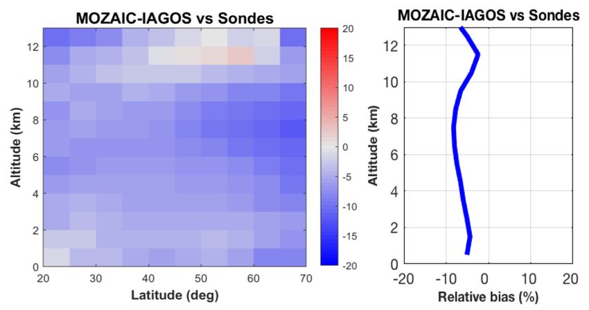
Tarasick et al: Tropospheric Ozone Assessment Report                                                   Art. 39, page 9 of 72

for non-chemists.” The Cauer method was used in multi-         ozone data is identifying the wavelengths and absorption
ple studies between 1935 and 1955 and in the national          cross-sections used. The values used for ozone absorp-
network of the then East Germany from 1952 until 1982          tion cross-sections in the Hartley and Huggins bands have
(Cauer 1951; Teichert 1955; Warmbt 1964; Feister and           changed with time, particularly up to the time of the
Warmbt 1987). It was compared with the Ehmert method           determination of Hearn (1961).
by Warmbt (1964). An initial study, with the two systems          To illustrate these variations, Table 3 extends in time
presumably in their normal operating conditions, gives a       and expands in wavelengths the information presented in
Cauer/Ehmert ratio of 0.66. A more intense study, stand-       the final table of Hearn (1961). Ozone absorption cross-
ardising various components and including blank correc-        sections are presented in units of cm2 molecule–1, with
tions gives a Cauer/Ehmert ratio of 0.90. However, for low     earlier units converted. Between 1913 and 2015 there is a
ozone concentrations, when the Cauer method measured           20% range in absorption cross-sections at 253.7 nm and a
less than 5 nmol mol–1, the Ehmert method often meas-          range that varies from
Table 3: (a) Absorption cross-sections of ozone [×1020 cm2 molecule–1] at selected Hg line wavelengths (in air). (b) Ratios relative to Gorshelev et al. (2014). DOI: https://doi.
  org/10.1525/elementa.376.t3

      Wavelength (nm)               253.65       263.30         265.20         269.90          275.20         280.40         289.36          292.50         296.73         302.15          302.50   312.50   334.15

      Fabry and Buisson (1931)        1046          917.0                –        779.9           582.8          361.7           175.7          116.6          66.85                   –    30.85    8.056    0.514
                                                                                                                                                                                                                      Art. 39, page 10 of 72

      Läuchli (1928)                  1277                –         1054                –               –        390.8                –              –         59.13                   –       –     8.227    0.600
      Ny and Choong (1933)            1222                –              –              –               –              –         185.1               –         70.19           31.88           –        –     0.574
      Vigroux (1953)                  1065                –              –              –               –              –         156.0               –         58.53          28.20            –        –     0.497
      Inn & Tanaka (1953)              1141         990.7          955.6          784.2           570.8          366.8           146.5          101.1          57.59          28.45         27.00    7.584    0.523
      Hearn (1961)                     1148               –              –              –               –              –         147.4               –         59.72          28.62            –        –     0.476
      Mauersberger et al. (1986)       1137               –              –              –               –              –              –              –               –                 –       –        –        –
      Malicet et al. (1995)            1131               –              –              –               –              –         151.3               –         61.46          29.85            –        –     0.466
      Gorshelev et al. (2014)          1122         988.9          939.1          806.2           582.5          386.8           153.8          106.0          61.59          30.36         28.58    7.279    0.493
      Viallon et al. (2015)            1127               –              –              –               –              –              –              –               –                 –       –        –        –
      Hodges et al. (2019)             1133

      Wavelength (nm)               253.65       263.30         265.20         269.90          275.20         280.40         289.36          292.50         296.73         302.15          302.50   312.50   334.15
      Fabry and Buisson (1931)         0.93          0.93            0.97           1.00           0.94            1.14            1.10           1.09               –          1.08         1.11     1.04     0.97
      Läuchli (1928)                   1.14              –           1.12               –              –           1.01               –              –           0.96                  –       –      1.13     1.22
      Ny and Choong (1933)             1.09              –               –              –              –               –          1.20               –           1.14           1.05           –        –      1.16
      Vigroux (1953)                   0.95              –               –              –              –               –          1.01               –           0.95           0.93           –        –      1.01
      Inn & Tanaka (1953)              1.02           1.00           1.02           0.97           0.98            0.95           0.95           0.95            0.94           0.94         0.94     1.04     1.06
      Hearn (1961)                     1.02              –               –              –              –               –          0.96               –           0.97           0.94           –        –      0.97
      Mauersberger et al. (1986)       1.01              –               –              –              –               –              –              –               –                 –       –        –        –
      Malicet et al. (1995)            1.01              –               –              –              –               –          0.98               –           1.00           0.98           –        –      0.95
      Gorshelev et al. (2014)             1               1              1              1              1               1              1              1               1                 1       1        1        1
      Viallon et al. (2015)            1.00              –               –              –              –               –              –              –               –                 –       –        –        –
      Hodges et al. (2019)             1.01
                                                                                                                                                                                                                      Tarasick et al: Tropospheric Ozone Assessment Report

                                        Downloaded from http://online.ucpress.edu/elementa/article-pdf/doi/10.1525/elementa.376/435292/376-6503-1-pb.pdf by guest on 05 January 2021
Tarasick et al: Tropospheric Ozone Assessment Report Art. 39, page 11 of 72
with the ozone reading of the analyser given in nmol mol–1. 2.2.3. Chemiluminescent methods of measuring tropospheric
Thus, at a mean level of 30 nmol mol–1 the total expanded ozone
uncertainty (95% confidence) is ±1.7 nmol mol–1. There are multiple chemiluminescent methods for meas-
A comparison of this bottom-up uncertainty analysis uring tropospheric ozone, of which the methods involving
with field results is shown in Figure 1 with the results ozone reaction with either ethylene, rhodamine B or nitric
of 559 calibrations of UV absorption photometers in oxide are relevant to this paper.
the Swiss National Air Pollution Monitoring Network. If The ethylene chemiluminescent ozone analyser (Warren
the assumptions for the uncertainty estimation are cor- and Babcock, 1970) is based on the reaction of ozone
rect, 95% of the calibration results shown in Figure 1 and ethylene, which produces electronically excited for-
should be found within the central part surrounded maldehyde. As this formaldehyde returns to the ground
by the grey shaded area. In fact, in Figure 1 less than state, light is emitted in a band centred at 430 nm, which
1.5% of the observed calibration results lie outside is detected by a photomultiplier. The count rate var-
the estimated uncertainty range, so for this extensive ies linearly with ozone concentration, provided the cell
dataset of UV absorption photometer field calibrations, pressure and temperature, the gain of the detector (the
Downloaded from http://online.ucpress.edu/elementa/article-pdf/doi/10.1525/elementa.376/435292/376-6503-1-pb.pdf by guest on 05 January 2021
the results fall well within the uncertainty estimate photomultiplier tube), the ethylene and sample flows and
(4). This reflects the robust nature of properly under- the composition of other components of the air sample
taken ozone measurements with the UV photometric are unchanged. The ethylene chemiluminescent ozone
method. analyser is a sensitive (~1 nmol mol–1) and stable instru-
The foregoing analysis does not cover all sources of ment with a fast response (~1 s) and importantly, is not
uncertainty, omitting those associated with such causes subject to SO2 or NO2 interference. The analyser requires
as inlet losses and potential interferences. The uncer- regular calibration with a standard ozone analyser, which
tainty of the absorption cross-section is not included, in the 1970s was either a KI or UV instrument. When
as the calibrations are performed with primary standard calibrated, the ethylene chemiluminescent analyser gives
analysers based on the same UV absorption cross-section. results that closely match those of the ultraviolet method
For the purposes of the subsequent analyses, at a mean as seen in the intercomparisons at Hohenpeissenberg,
level of 30 nmol mol–1, the total expanded uncertainty Germany (Attmannspacher and Hartmannsgruber 1982)
(95% confidence) in modern ozone measurements is and Cape Grim, Australia (Elsworth and Galbally 1984).Art. 39, page 12 of 72 Tarasick et al: Tropospheric Ozone Assessment Report photomultiplier tube), the nitric oxide and sample flows Criterion 2: It is known that SO2 causes quantitative and the composition of other components of the air sam- negative interference with the KI measurement meth- ple are unchanged. The nitric oxide chemiluminescent ods (Albert-Lévy, 1907; Glückauf, 1941, 1944; Saltzman ozone analyser is a stable instrument with a sensitive and Gilbert 1959a), with a stoichiometry reported as 1.0 (~0.1 nmol mol–1) and fast response (~1 s) and not sub- (Schenkel and Broder, 1982; Volz and Kley, 1988). SO2 is ject to SO2 or NO2 interference. A current description of known to be present in very low concentrations in the the instrument is available (Campos et al., 2006). The ana- background atmosphere of
Tarasick et al: Tropospheric Ozone Assessment Report Art. 39, page 13 of 72
the measurements appear to be of excellent quality and 3.1. The Montsouris Observatory ozone measurements
well documented, except that they differ by a factor of 1876–1910
100 from current measurements. As Fabry (1950) said, the The ozone measurements at the Municipal Observatory
results are absurd. Serious artifacts and inconsistencies at the Parc de Montsouris at the southern edge of Paris
associated with individual datasets are discussed in the (Albert-Lévy, 1877) from 1876–1910, are the oldest active
Supplemental Material (Text S-3). sampling ozone measurements known. As noted in Sec-
For every site, the method used, the possible pollu- tion 2.1.1, they are pivotal to conclusions in previous work
tion sources, the topography, surface cover and prevail- that ozone in pre-industrial times was much less than its
ing meteorology and credibility of the results have been present concentration (e.g. Marenco et al., 1994). Hence
examined to assess the suitability of the observations the Montsouris observations are examined in detail here.
for inclusion in the historical record. One excluded site The technique used was the KI-arsenite system and is
is explicitly included in the following discussion. This is related to the UV method as described in Section 2.1.2,
Montsouris, Paris, which is discussed here because it has and is a valid method.
been used as a central set of data for a number of previ- Volz and Kley (1988) examined daily measurements
Downloaded from http://online.ucpress.edu/elementa/article-pdf/doi/10.1525/elementa.376/435292/376-6503-1-pb.pdf by guest on 05 January 2021
ous historical reconstructions of tropospheric ozone. For of ozone at Montsouris in 1876–86 and 1905 and corre-
the other historical data discussed below, in all cases the lated the results with the wind direction. The area to the
method is valid and with one exception, the sites are pre- southwest of Montsouris had no significant urban centers
sumed free of interfering pollutants and representative of in 1876–1905 and Volz and Kley concluded that air from
the well-mixed boundary layer. In a few cases some of the the southwest would be free of urban air pollutants which
data are excluded on credibility grounds, and some are might interfere with the analysis. It was found that with
accepted with caution; the reasons for these decisions are wind from the southwest the average ozone levels meas-
discussed. Before discussing the available historical data ured in 1876–86 and 1905 were approximately 8 and 10
which passed the selection criteria, it is worth repeating nmol mol–1, and with wind from directions other than
the cautionary note from Section 2: for comparison with southwest the ozone levels were lower by 2 and 5 nmol
current observations these data should be treated as a mol–1, respectively. The lower ozone levels observed when
group, because there are substantial unknown uncertain- the wind direction was from Paris were attributed to the
ties associated with the bias corrections of each individual presence of SO2 in the Paris urban plume. The corrected
set of observations. ozone data gave an average ozone level of 11 nmol mol–1
There are some other features of the data that are over the period 1876–1910 (Volz and Kley 1988). This is
important to note. Some studies involve measurements much lower than that found at clean mid-latitude sites
at multiple sites; other studies have long records at one today.
site that have been broken into distinct periods. Thus the Observers in the 19th century were aware of the poten-
number of published studies and the number of data sets tial for interference of reducing gases with the KI reaction,
do not correspond. The 60 data sets accepted into the and, as noted by Volz and Kley (1988), an attempt was
record, their site names, locations, data references etc. are made to quantify these interferences. Average values for
presented in Tables 4, 5 and 6. During the period 1870s 1905–07 of “gaz réducteurs” correspond to ~3 nmol mol–1,
–1950, most of the available measurements were made with weekly values as high as 16 nmol mol–1 (Albert-Lévy,
using KI techniques with a small number of spectroscopic 1907, 1908). However, exactly how to interpret these
measurements by UV absorption. The studies were occa- measurements remains uncertain, as SO2 does not react
sional scientific experiments, usually of limited duration strongly with KI in the absence of ozone.
and initially in central and northern Europe. From 1950 The period 1870s to 1900s was one of rapid change in
to the 1970s the coverage became global and measure- Paris. During the period 1870–1880, Paris was a city of
ments at a given location moved to yearly or greater 2 million people and coal supplied 58% and wood 42%
duration. of the city’s total energy needs (Kim and Barles, 2012).
The standard deviations presented here differ for the Coal burning releases SO2, and two approaches are taken
periods 1890–1950 and 1950–1970 because of the pau- to estimate SO2 in Paris at this time. Firstly, measure-
city of data in the earlier period. In the period 1890–1950 ments of ambient SO2 in Paris began in the 1950s, and
the standard deviation is calculated from daily ozone val- records of coal use in the city are available from 1875.
ues when there are 7 or more days of data. In the period These concentration and emission data are combined to
1950–1970 the standard deviation is calculated from the estimate SO2 levels of 55 nmol mol–1 in Paris in the early
monthly mean ozone values for an annual cycle or longer 20th century (Ionescu et al., 2012). However, this approach
when there is at least one year of data. For more informa- neglects activities outside the city boundary where both
tion see the Supplemental Material (Text S-5). building construction and the presence of gasworks
The observations are grouped into the tropical (0°–30°), that provided gas to Paris were located (Kim and Barles,
temperate (30°–60°) and polar (60°–90°) regions of each 2012; Kesztembaum and Rosenthal 2014). Secondly, at
hemisphere. They are presented in Tables 4–6 and dis- Montsouris measurements were made of sulphate in rain-
cussed in the following text for different periods. Ozone is water with an average of 13.9 mg l–1 (range 3.5–37.0 mg
summarized for each region using a weighted mean, with l–1) as SO3–1: (Albert-Lévy, 1907, 1908). Sulphate in rainwa-
the weighting proportional to the number of days with ter is closely associated with atmospheric sulphur dioxide,
observations at each site. and such sulphate values are typical of highly pollutedYou can also read