Market Basket Analysis and Mining Association Rules
←
→
Page content transcription
If your browser does not render page correctly, please read the page content below
Market Basket Analysis
          and
Mining Association Rules

                           1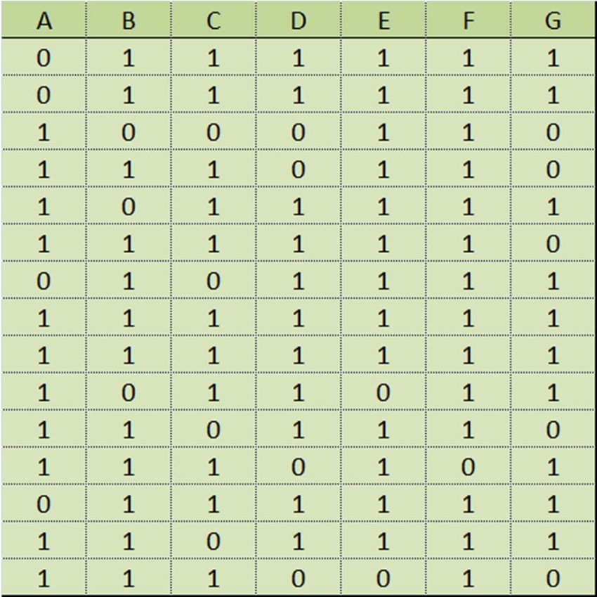
Mining Association Rules
Market Basket Analysis
What is Association rule mining
Apriori Algorithm
Measures of rule interestingness
2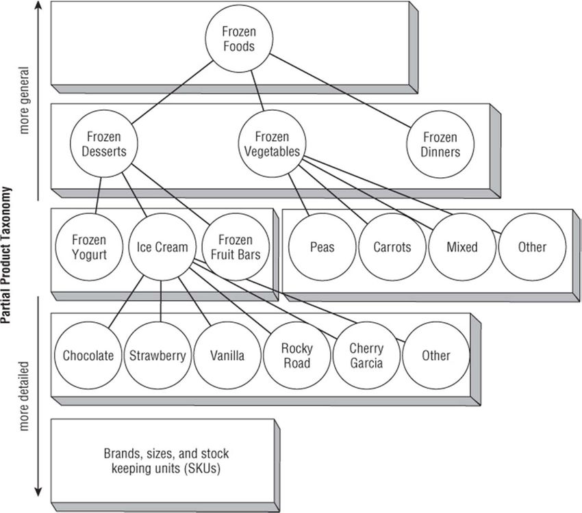
Market Basket Analysis
One basket tells you about
what one customer purchased
at one time.
A loyalty card makes it possible
to tie together purchases by a
single customer (or household)
over time.
3
Market Basket Analysis
Retail – each customer purchases different set of products,
different quantities, different times
MBA uses this information to:
Identify who customers are (not by name)
Understand why they make certain purchases
Gain insight about its merchandise (products):
Fast and slow movers
Products which are purchased together
Products which might benefit from promotion
Take action:
Store layouts
Which products to put on specials, promote, coupons…
Combining all of this with a customer loyalty card it becomes
even more valuable
more than just the contents of shopping carts
It is also about what customers do not purchase, and why.
If customers purchase baking powder, but no flour, what are they
baking?
If customers purchase a mobile phone, but no case, are you
missing an opportunity?
It is also about key drivers of purchases; for example, the
gourmet mustard that seems to lie on a shelf collecting dust until
a customer buys that particular brand of special gourmet mustard
in a shopping excursion that includes hundreds of dollars' worth
of other products. Would eliminating the mustard (to replace it
with a better‐selling item) threaten the entire customer
relationship?
5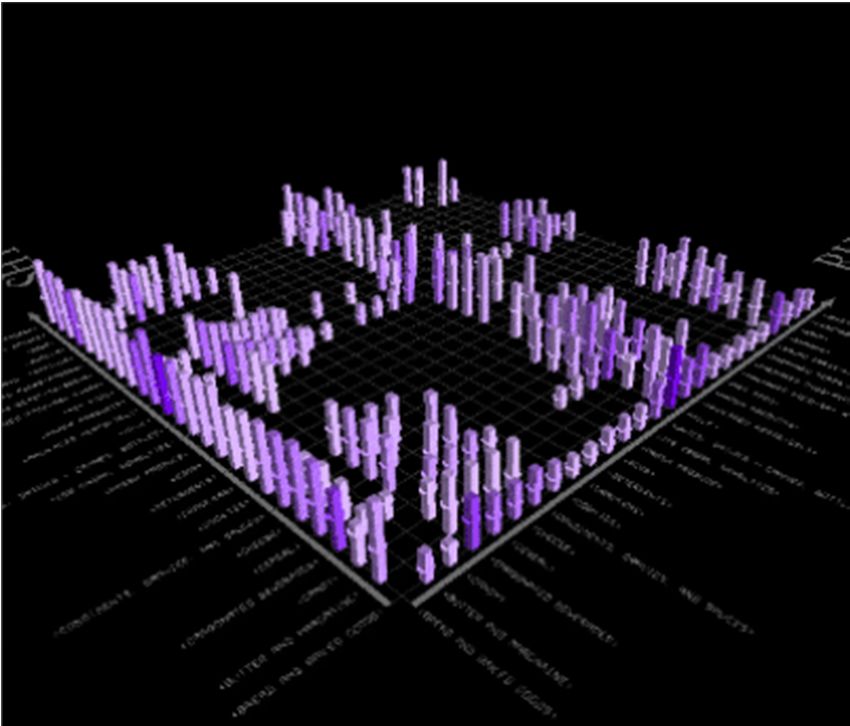
Market Basket Analysis
association rules can be applied on other types of “baskets.”
Items purchased on a credit card, such as rental cars and hotel rooms,
provide insight into the next product that customers are likely to purchase,
Optional services purchased by telecommunications customers (call
waiting, call forwarding, DSL, speed call, and so on) help determine how to
bundle these services together to maximize revenue.
Banking products used by retail customers (money market accounts,
certificate of deposit, investment services, car loans, and so on) identify
customers likely to want other products.
Unusual combinations of insurance claims can be a sign of fraud and can
spark further investigation.
Medical patient histories can give indications of likely complications based
on certain combinations of treatments.
6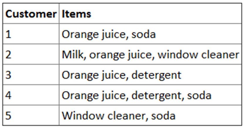
Market Basket Analysis
The order is the fundamental data structure for market basket
data. An order represents a single purchase event by a customer.
The customer entity is optional and should be available when a
customer can be identified over time.
Tracking customers over time makes it possible to determine, for
instance, which grocery shoppers “bake from scratch”
interesting to the makers of flour as well as prepackaged cake mixes and
the makers of aprons and kitchen appliances.
The store entity provides information about where the products
are purchased.
7
Market Basket Analysis: Basic Measures
Ex. of questions to ask before starting with fancy techniques:
Average number of orders per customer
Change in average number of orders per customer over time
Average number of unique items per order
Change in average number of unique items per order over time
Proportion of customers and average purchase size of customers who
purchase the most popular products
Proportion of customers and average purchase size of customers who
purchase the least popular products
Average order size
Changes in average order size over time
Average order size by important dimensions, such as geography, method of
payment, time of year, and so on
8
In some cases, few customers have multiple purchases, so the proportion of
orders per customer is close to one, suggesting a business opportunity to
increase the number of sales per customer.
The Figure represents the number of unique items ever purchased by the
depth of the relationship (the number of orders) for customers who purchased
more than one item from a small specialty retailer.
9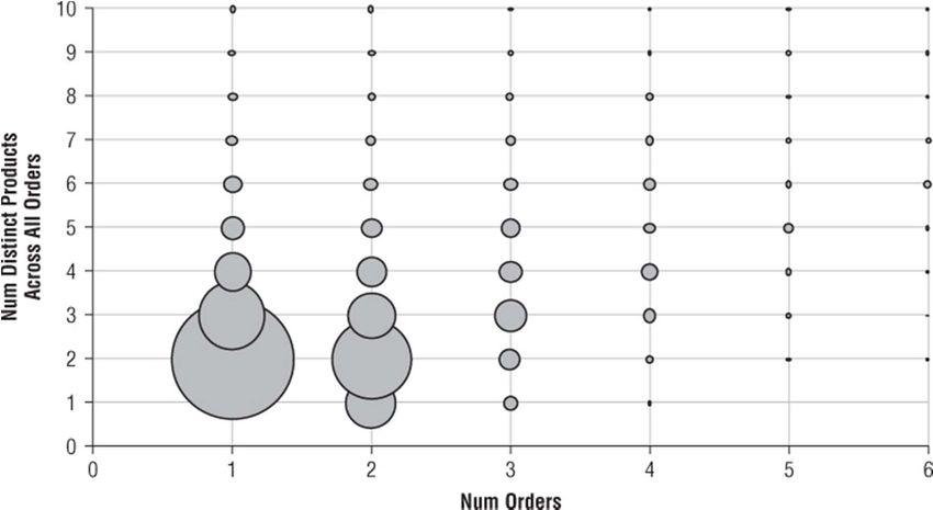
Tracking Marketing Interventions
10Mining Association Rules
Market Basket Analysis
What is Association rule mining
Apriori Algorithm
Measures of rule interestingness
11What Is Association Rule Mining?
Association rule mining
Finding frequent patterns, associations, correlations, or causal
structures among sets of items in transaction databases
Understand customer buying habits by finding associations and
correlations between the different items that customers place in their
“shopping basket”
Applications
Basket data analysis, cross‐marketing, catalog design, loss‐leader
analysis, web log analysis, fraud detection (supervisor‐>examiner)
12How can Association Rules be used?
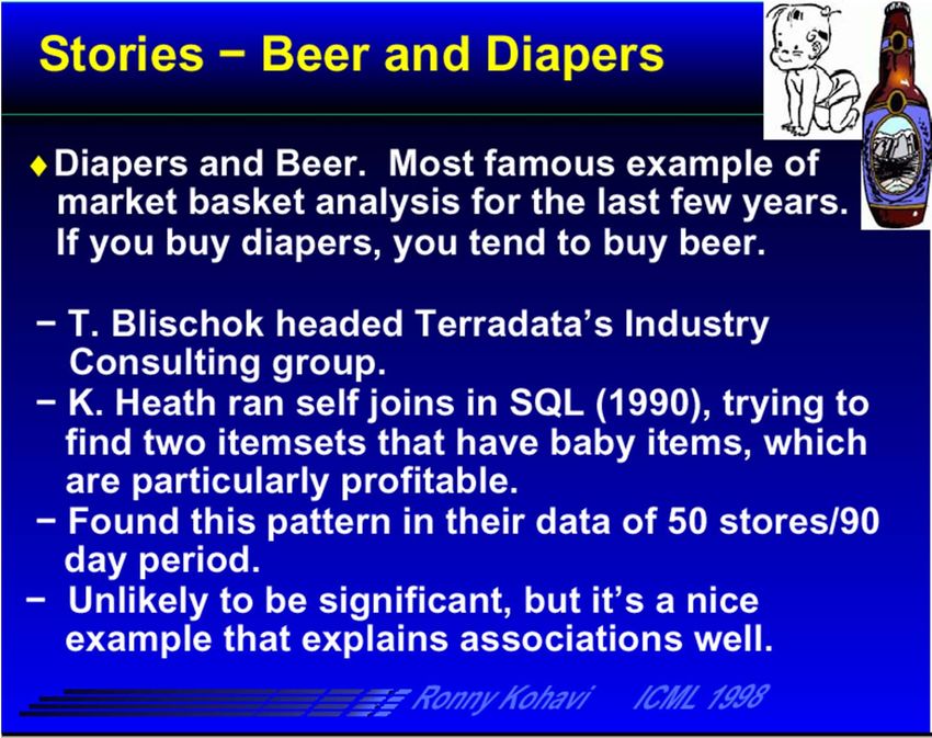
Probably mom was
calling dad at work to
buy diapers on way
home and he
decided to buy a six‐
pack as well.
The retailer could
move diapers and
beers to separate
places and position
high‐profit items of
interest to young
fathers along the
path.
13What Is Association Rule Mining?
Rule form
Antecedent Consequent [support, confidence]
(support and confidence are user defined measures of interestingness)
Examples
buys(x, “computer”) buys(x, “financial management
software”) [0.5%, 60%]
age(x, “30..39”) ^ income(x, “42..48K”) buys(x, “car”)
[1%,75%]
14How can Association Rules be used?
Let the rule discovered be
{Bagels,...} {Potato Chips}
Potato chips as consequent => Can be used to determine what should
be done to boost its sales
Bagels in the antecedent => Can be used to see which products would
be affected if the store discontinues selling bagels
Bagels in antecedent and Potato chips in the consequent => Can be
used to see what products should be sold with Bagels to promote sale
of Potato Chips
15Orange juice and soda are more likely to be purchased together than any other
two items.
Detergent is never purchased with window cleaner or milk.
Milk is never purchased with soda or detergent.
16Association rule types
Actionable Rules
contain high‐quality, actionable information
Trivial Rules
information already well‐known by those familiar with the
business
Inexplicable Rules
no explanation and do not suggest action
Trivial and Inexplicable Rules occur most often
17Rules
Wal‐Mart customers who purchase Barbie dolls have a
60% likelihood of also purchasing one of three types of
candy bars [Forbes, Sept 8, 1997]
Customers who purchase maintenance agreements are
very likely to purchase large appliances (Linoff and Berry
experience)
When a new hardware store opens, one of the most
commonly sold items is toilet bowl cleaners (Linoff and
Berry experience)
18Basic Concepts
Given:
(1) database of transactions,
(2) each transaction is a list of items purchased by a
customer in a visit
Find:
all rules that correlate the presence of one set of items
(itemset) with that of another set of items
E.g., 35% of people who buys salmon also buys cheese
19Rule Basic Measures
A B [ s, c ]
Support: denotes the frequency of the rule within transactions. A
high value means that the rule involves a great part of database.
support(A B [ s, c ]) = p(A B)
Confidence: denotes the percentage of transactions containing A
which also contain B. It is an estimation of conditioned probability .
confidence(A B [ s, c ]) = p(B|A) = sup(A,B)/sup(A).
20Tr1 Shoes, Socks, Tie, Belt
Tr2 Shoes, Socks, Tie, Belt, Shirt, Hat
Tr3 Shoes, Tie
Tr4 Shoes, Socks, Belt
Transaction Shoes Socks Tie Belt Shirt Scarf Hat
1 1 1 1 0 0 0
2 1 1 1 1 1 0 1
3 1 0 1 0 0 0 0
4 1 1 0 1 0 0 0
...
Support is 50% (2/4)
Socks Tie Confidence is 66.67% (2/3)
21transactions
Rule C => D support
confidence /
22Example Definitions:
Trans. Id Purchased Items Itemset:
1 A,D A,B or B,E,F
2 A,C Support of an itemset:
3 A,B,C Sup(A,B)=1
4 B,E,F Sup(A,C)=2
Frequent pattern:
Given min. sup=2, {A,C} is a
frequent pattern
For minimum support = 50% and minimum confidence = 50%, we have the
following rules
A => C with 50% support and 66% confidence
C => A with 50% support and 100% confidence
23Other Applications
“Baskets” = documents
“items” = words in those documents
Lets us find words that appear together unusually frequently,
i.e., linked concepts.
Word 1 Word 2 Word 3 Word 4
Doc 1 1 0 1 1
Doc 2 0 0 1 1
Doc 3 1 1 1 0
Word 4 => Word 3
When word 4 occurs in a document there a big probability of word 3
occurring
24Other Applications
“Baskets” = sentences
“items” = documents containing those sentences
Items that appear together too often could represent
plagiarism.
Doc 1 Doc 2 Doc 3 Doc 4
Sent 1 1 0 1 1
Sent 2 0 0 1 1
Sent 3 1 1 1 0
Doc 4 => Doc 3
When a sentence occurs in document 4 there is a big probability of
occurring in document 3
25Other Applications
“Baskets” = Web pages;
“items” = linked pages.
Pairs of pages with many common references may be about
the same topic.
“Baskets” = Web pages pi ;
“items” = pages that link to pi
Pages with many of the same links may be mirrors or about
the same topic. wp a wp b wp c wp d
wp1
wp2
26Randall Matignon 2007, Data Mining Using SAS Enterprise Miner, Wiley (book).
27The support probability of each rule is identified by the color of the symbols and the confidence probability
of each rule is identified by the shape of the symbols. The items that have the highest confidence are
Heineken beer, crackers, chicken, and peppers.
Randall Matignon 2007, Data Mining Using SAS Enterprise Miner, Wiley (book).
2829
Mining Association Rules
Market Basket Analysis
What is Association rule mining
Apriori Algorithm
Measures of rule interestingness
30Boolean association rules
Each transaction is
converted to a
Boolean vector
31Finding Association Rules
Approach:
1) Find all itemsets that have high support
‐ These are known as frequent itemsets
2) Generate association rules from frequent itemsets
32Itemset Lattice for 5 products
null
A B C D E
AB AC AD AE BC BD BE CD CE DE
ABC ABD ABE ACD ACE ADE BCD BCE BDE CDE
ABCD ABCE ABDE ACDE BCDE
ABCDE
33Apriori principle
Any subset of a frequent itemset must be
frequent
A transaction containing {beer, diaper, nuts} also contains
{beer, diaper}
{beer, diaper, nuts} is frequent {beer, diaper} must also
be frequent
34Apriori principle
No superset of any infrequent itemset should be
generated or tested
Many item combinations can be pruned
35Apriori principle for pruning candidates
If an itemset is infrequent, null
then all of its supersets must
also be infrequent A B C D E
AB AC AD AE BC BD BE CD CE DE
Found to be
Infrequent ABC ABD ABE ACD ACE ADE BCD BCE BDE CDE
Pruned ABCD ABCE ABDE ACDE BCDE
supersets
ABCDE
36Mining Frequent Itemsets (the Key Step)
Find the frequent itemsets: the sets of items that
have (at least) minimum support
A subset of a frequent itemset must also be a frequent
itemset
Generate length (k+1) candidate itemsets from length
k frequent itemsets, and
Test the candidates against DB to determine which are
in fact frequent
37How to Generate Candidates? ‐ step 1
The items in Lk‐1 are listed in an order
Step 1: self‐joining Lk‐1
insert into Ck
select p.item1, p.item2, …, p.itemk‐1, q.itemk‐1
from Lk‐1 p, Lk‐1 q
where p.item1=q.item1, …, p.itemk‐2=q.itemk‐2, p.itemk‐1 < q.itemk‐1
A D E
=
=
<
A D F
38L3 – set of itemsets of size 3 that are frequent
(itemsets need to be sorted)
itemset 1 A B C
itemset 2 A D E
A,D,E,F
itemset 3 A D F
itemset 4 A E F
Two itemsets with the same k‐1 = 3‐1 elements are merged and inserted in
C4 (the set of candidate itemsets of size 4).
Those in C4 that have support above the threshold are inserted in L4.
39The Apriori Algorithm — Example
Min. support: 2 transactions
Database D C1 itemset sup.
TID Items {1} 2 L1 itemset sup.
100 134 {2} 3 {1} 2
200 235 Scan D {3} 3 {2} 3
300 1235 {4} 1 {3} 3
400 25 {5} 3 {5} 3
C2 itemset sup C2 itemset
L2 itemset sup {1 2} 1 {1 2}
{1 3} 2 {1 3} 2 {1 3}
{2 3} 2 {1 5} 1 Scan D {1 5}
{2 3} 2 {2 3}
{2 5} 3
{2 5} 3 {2 5}
{3 5} 2
{3 5} 2 {3 5}
C3 itemset Scan D L3 itemset sup
{2 3 5} {2 3 5} 2
40How to Generate Candidates? – step 2
Step 2: pruning
for all itemsets c in Ck do
for all (k‐1)‐subsets s of c do
if (s is not in Lk‐1) then delete c from Ck
A D E F
Note: In step 1 we may generate candidates that include itemsets of size k‐1 that
are not frequent.
The pruning step may be able to eliminate some candidates without counting
their support.
Counting support is a computationally demanding task. 41Example of Generating Candidates – step 1
L3 = {abc, abd, acd, ace, bcd}
Self‐joining: L3*L3
joining abc and abd gives abcd
joining acd and ace gives acde
42Example of Generating Candidates – step 2
L3 = {abc, abd, acd, ace, bcd}
Pruning (before counting its support):
abcd: check if abc, abd, acd, bcd, are in L3
acde: check if acd, ace, ade, cde are in L3
acde is removed because ade is not in L3
Thus C4={abcd}
43The Apriori Algorithm
Ck: Candidate itemset of size k Lk : frequent itemset of size k
Join Step: Ck is generated by joining Lk‐1 with itself
Prune Step: Any (k‐1)‐itemset that is not frequent cannot be a subset of a
frequent k‐itemset
Algorithm:
L1 = {frequent items};
for (k = 1; Lk !=; k++) do begin
Ck+1 = candidates generated from Lk;
for each transaction t in database do
increment the count of all candidates in Ck+1 that are
contained in t
Lk+1 = candidates in Ck+1 with min_support
end
return L = k Lk;
44Generating AR from frequent intemsets
Confidence (AB) = P(B|A) = support_count({A, B})
support_count({A})
For every frequent itemset x, generate all non‐empty
subsets of x
For every non‐empty subset s of x, output the rule
“ s (x‐s) ” if
support_count({x})
min_conf
support_count({s})
45Rule Generation
How to efficiently generate rules from frequent
itemsets?
In general, confidence does not have an anti‐monotone
property
But confidence of rules generated from the same itemset has
an anti‐monotone property
L = {A,B,C,D}:
c(ABC D) c(AB CD) c(A BCD)
Confidence is non‐increasing as number of items in rule
consequent increases
46From Frequent Itemsets to Association Rules
Q: Given frequent set {A,B,E}, what are
possible association rules?
A => B, E
A, B => E
A, E => B
B => A, E
B, E => A
E => A, B
__ => A,B,E (empty rule), or true => A,B,E
47Generating Rules: example
Trans-ID Items Min_support: 60%
1 ACD Min_confidence: 75%
2 BCE
3 ABCE
4 BE
5 ABCE Frequent Itemset Support
{BCE},{AC} 60%
Rule Conf. {BC},{CE},{A} 60%
{BC} =>{E} 100% {BE},{B},{C},{E} 80%
{BE} =>{C} 75%
{CE} =>{B} 100%
{B} =>{CE} 75%
{C} =>{BE} 75%
{E} =>{BC} 75%
48Exercice
TID Items
1 Bread, Milk, Chips, Mustard
2 Beer, Diaper, Bread, Eggs Converta os dados para o
3 Beer, Coke, Diaper, Milk formato booleano e para um
suporte de 40%, aplique o
4 Beer, Bread, Diaper, Milk, Chips algoritmo apriori.
5 Coke, Bread, Diaper, Milk
6 Beer, Bread, Diaper, Milk, Mustard
7 Coke, Bread, Diaper, Milk
Bread Milk Chips Mustard Beer Diaper Eggs Coke
1 1 1 1 0 0 0 0
1 0 0 0 1 1 1 0
0 1 0 0 1 1 0 1
1 1 1 0 1 1 0 0
1 1 0 0 0 1 0 1
1 1 0 1 1 1 0 0
1 1 0 0 0 1 0 1
490.4*7= 2.8
C1 L1 C2 L2
Bread 6 Bread 6 Bread,Milk 5 Bread,Milk 5
Milk 6 Milk 6 Bread,Beer 3 Bread,Beer 3
Chips 2 Beer 4 Bread,Diaper 5 Bread,Diaper 5
Mustard 2 Diaper 6 Bread,Coke 2 Milk,Beer 3
Beer 4 Coke 3 Milk,Beer 3 Milk,Diaper 5
Diaper 6 Milk,Diaper 5 Milk,Coke 3
Eggs 1 Milk,Coke 3 Beer,Diaper 4
Coke 3 Beer,Diaper 4 Diaper,Coke 3
Beer,Coke 1
Diaper,Coke 3
C3 L3
Bread,Milk,Beer 2 Bread,Milk,Diaper 4
Bread,Milk,Diaper 4 Bread,Beer,Diaper 3
Bread,Beer,Diaper 3 Milk,Beer,Diaper 3
Milk,Beer,Diaper 3 Milk,Diaper,Coke 3
Milk,Beer,Coke
Milk,Diaper,Coke 3
8 C 28 C 38 92 24
50Mining Association Rules
Market Basket Analysis
What is Association rule mining
Apriori Algorithm
Measures of rule interestingness
51Interestingness Measurements
How good is the association Rule?
Are all of the strong association rules discovered interesting
enough to present to the user?
How can we measure the interestingness of a rule?
Subjective measures
A rule (pattern) is interesting if
• it is unexpected (surprising to the user); and/or
• actionable (the user can do something with it)
• (only the user can judge the interestingness of a rule)
52Objective measures of rule interest
Support
Confidence or strength
Lift or Interest or Correlation
Conviction
Leverage or Piatetsky‐Shapiro
53Criticism to Support and Confidence
Example 1: (Aggarwal & Yu, PODS98)
Among 5000 students basketball not basketball sum(row)
cereal 2000 1750 3750 75%
3000 play basketball
not cereal 1000 250 1250 2 5%
3750 eat cereal sum(col.) 3000 2000 5000
60% 40%
2000 both play basket
ball and eat cereal
play basketball eat cereal [40%, 66.7%]
misleading because the overall percentage of students eating cereal is 75% which
is higher than 66.7%.
play basketball not eat cereal [20%, 33.3%]
is more accurate, although with lower support and confidence
54Lift of a Rule
sup(A, B) p(B|A)
LIFT(A B)
sup(A)sup(B) p(B)
2000
LIFT 5000 0.89
play basketball eat cereal [40%, 66.7%] 3000 3750
5000 5000
1000
LIFT 5000 1.33
play basketball not eat cereal [20%, 33.3%] 3000 1250
5000 5000
basketball not basketball sum(row)
cereal 2000 1750 3750
not cereal 1000 250 1250
sum(col.) 3000 2000 5000
55Problems With Lift
Rules that hold 100% of the time may not have the highest
possible lift. For example, if 5% of people are Vietnam veterans
and 90% of the people are more than 5 years old, we get a lift of
0.05/(0.05*0.9)=1.11 which is only slightly above 1 for the rule
Vietnam veterans ‐> more than 5 years old.
And, lift is symmetric:
not eat cereal play basketball [20%, 80%]
1000
LIFT 5000 1.33
1250 3000
5000 5000
56Conviction of a Rule
sup(A) sup(B) P(A) P(B) P(A)(1 P(B))
Conv (A B)
sup(A, B) P(A,B) P(A) P(A, B)
Conviction is a measure of the implication and has value 1 if items are unrelated.
3000 3750
1
5000 5000
play basketball eat cereal [40%, 66.7%] Conv
3000 2000
0.75
eat cereal play basketball conv:0.85 5000 5000
3000 1250
play basketball not eat cereal [20%, 33.3%] 1
5000
5000
Conv 1.125
not eat cereal play basketball conv:1.43 3000 1000
5000 5000
57Conviction
conviction of X=>Y can be interpreted as the
ratio of the expected frequency that X occurs without Y (that is to
say, the frequency that the rule makes an incorrect prediction) if
X and Y were independent
divided by the observed frequency of incorrect predictions.
A conviction value of 1.2 shows that the rule would be incorrect
20% more often (1.2 times as often) if the association between X
and Y was purely random chance.
58Leverage of a Rule
Leverage or Piatetsky‐Shapiro
PS(A B) sup(A, B) sup(A) sup(B)
PS (or Leverage):
is the proportion of additional elements covered by both the
premise and consequence above the expected if independent.
59Comments
Traditional methods such as database queries:
support hypothesis verification about a relationship such as
the co‐occurrence of diapers & beer.
Data Mining methods automatically discover significant
associations rules from data.
Find whatever patterns exist in the database, without the
user having to specify in advance what to look for (data
driven).
Therefore allow finding unexpected correlations
60Choosing the Right Set of Items
61Product Hierarchies Help to Generalize Items
Are large fries and small fries the same product?
Is the brand of ice cream more relevant than its flavor?
Which is more important: the size, style, pattern, or designer
of clothing?
Is the energy‐saving option on a large appliance indicative of
customer behavior?
Market basket analysis produces the best results when the items occur in
roughly the same number of transactions in the data. This helps prevent
rules from being dominated by the most common items. Product
hierarchies can help here. Roll up rare items to higher levels in the
hierarchy, so they become more frequent. More common items may not
have to be rolled up at all.
6263
Virtual Items Go Beyond the Product Hierarchy
The purpose of virtual items is to enable the analysis to take
advantage of information that goes beyond the product
hierarchy.
Examples of virtual items might be
designer labels, such as Calvin Klein, that appear in both apparel
departments and perfumes
low‐fat and no‐fat products in a grocery store
energy‐saving options on appliances
whether the purchase was made with cash, a credit card, or check
the day of the week or the time of day the transaction occurred
virtual items can also be used to specify which group, such as an existing
location or a new location, generates the transaction.
64Application Difficulties
Wal‐Mart knows that customers who buy Barbie dolls (it
sells one every 20 seconds) have a 60% likelihood of
buying one of three types of candy bars. What does
Wal‐Mart do with information like that?
'I don't have a clue,' says Wal‐Mart's chief of
merchandising, Lee Scott.
See ‐ KDnuggets 98:01 for many ideas
www.kdnuggets.com/news/98/n01.html
65Some Suggestions
By increasing the price of Barbie doll and giving the type of candy bar free, wal‐mart
can reinforce the buying habits of that particular types of buyer
Highest margin candy to be placed near dolls.
Special promotions for Barbie dolls with candy at a slightly higher margin.
Take a poorly selling product X and incorporate an offer on this which is based on
buying Barbie and Candy. If the customer is likely to buy these two products anyway
then why not try to increase sales on X?
Probably they can not only bundle candy of type A with Barbie dolls, but can also
introduce new candy of Type N in this bundle while offering discount on whole bundle.
As bundle is going to sell because of Barbie dolls & candy of type A, candy of type N can
get free ride to customers houses. And with the fact that you like something, if you see
it often, Candy of type N can become popular.
66References
Jiawei Han and Micheline Kamber, “Data Mining: Concepts and
Techniques”, 2 edition (4 Jun 2006),
Gordon S. Linoff and Michael J. Berry, “Data Mining Techniques:
For Marketing, Sales, and Customer Relationship Management”,
3rd Edition edition (1 April 2011)
Vipin Kumar and Mahesh Joshi, “Tutorial on High Performance
Data Mining ”, 1999
Rakesh Agrawal, Ramakrishnan Srikan, “Fast Algorithms for
Mining Association Rules”, Proc VLDB, 1994
(http://www.cs.tau.ac.il/~fiat/dmsem03/Fast%20Algorithms%20for%20Mining%20Association%20Rules.ppt)
67You can also read