Meta-analysis of Cryogenian through modern quartz microtextures reveals
←
→
Page content transcription
If your browser does not render page correctly, please read the page content below
ESSOAr | https://doi.org/10.1002/essoar.10504352.2 | CC_BY_4.0 | First posted online: Sun, 16 May 2021 17:05:40 | This content has not been peer reviewed.

                              Confidential manuscript submitted to the Journal of Sedimentary Research (JSR)

                      Meta-analysis of Cryogenian through modern quartz microtextures reveals
                                            sediment transport histories
                      Jocelyn N. Reahl1, 2, Marjorie D. Cantine1, Julia Wilcots1, Tyler J. Mackey1, 3, Kristin D.
                                                             Bergmann1

                        1
                        Massachusetts Institute of Technology, Department of Earth, Atmospheric, and Planetary
                                           Sciences, Cambridge, Massachusetts, 02139, U.S.A.
                     2
                       Now at the California Institute of Technology, Division of Geological and Planetary Sciences,
                                                    Pasadena, California, 91125, U.S.A.
                          3
                            Now at the University of New Mexico, Department of Earth and Planetary Sciences,
                                                Albuquerque, New Mexico, 87131, U.S.A.

                                          Corresponding author: Jocelyn N. Reahl (jreahl@caltech.edu)

                                                                                                                                               1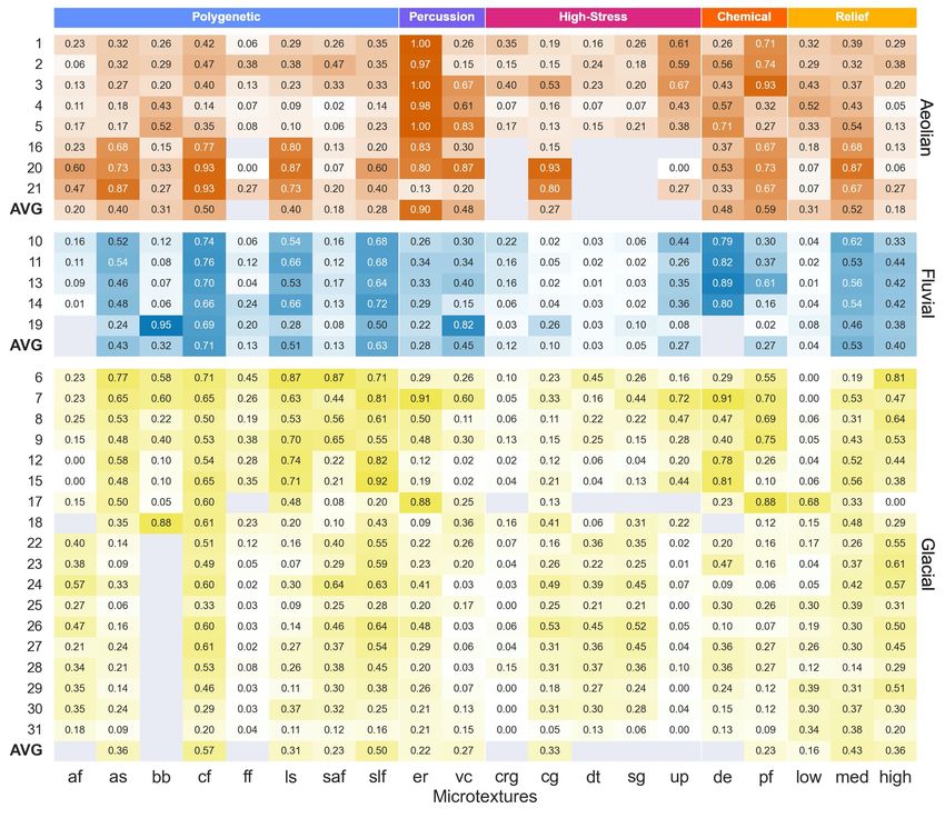
ESSOAr | https://doi.org/10.1002/essoar.10504352.2 | CC_BY_4.0 | First posted online: Sun, 16 May 2021 17:05:40 | This content has not been peer reviewed.

                              Confidential manuscript submitted to the Journal of Sedimentary Research (JSR)

             1                                                           ABSTRACT

             2               Quantitative scanning electron microscopy (SEM) quartz microtextural analysis can

             3     reveal the transport histories of modern and ancient sediments. However, because workers

             4     identify and count microtextures differently, it is difficult to directly compare quantitative

             5     microtextural data analyzed by different workers. As a result, the defining microtextures of

             6     certain transport modes and their probabilities of occurrence are not well constrained. We used

             7     principal component analysis (PCA) to directly compare modern and ancient aeolian, fluvial, and

             8     glacial samples from the literature with 9 new samples from active aeolian and glacial

             9     environments. Our results demonstrate that PCA can group microtextural samples by transport

           10      mode and differentiate between aeolian and fluvial/glacial transport modes across studies. The

           11      PCA ordination indicates that aeolian samples are distinct from fluvial and glacial samples,

           12      which are in turn difficult to disambiguate from each other. Ancient and modern sediments are

           13      also shown to have quantitatively similar microtextural relationships. Therefore, PCA may be a

           14      useful tool to constrain the ambiguous transport histories of some ancient sediment grains. As a

           15      case study, we analyzed two samples with ambiguous transport histories from the Cryogenian

           16      Bråvika Member (Svalbard). Integrating PCA with field observations, we find evidence that the

           17      Bråvika Member facies investigated here includes aeolian deposition and may be analogous to

           18      syn-glacial Marinoan aeolian units including the Bakoye Formation in Mali and the Whyalla

           19      Sandstone in South Australia.

           20

           21                                                        INTRODUCTION

           22                Scanning electron microscopy (SEM) quartz microtextural analysis reveals microscale

           23      features (microtextures) that are formed during transport (Krinsley and Takahashi 1962; Krinsley

                                                                                                                                               2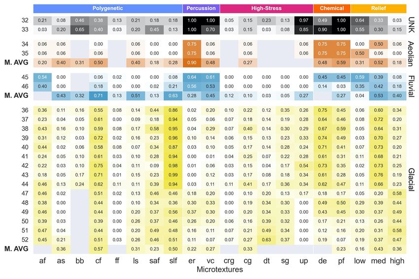
ESSOAr | https://doi.org/10.1002/essoar.10504352.2 | CC_BY_4.0 | First posted online: Sun, 16 May 2021 17:05:40 | This content has not been peer reviewed.

                              Confidential manuscript submitted to the Journal of Sedimentary Research (JSR)

           24      and Doornkamp 1973; Bull 1981). Because different transport modes imprint specific suites of

           25      microtextures onto quartz grains, quartz microtextural analysis is a useful technique to

           26      understand the transport histories of modern and ancient sedimentary deposits (Krinsley and

           27      Doornkamp 1973; Mahaney 2002; Vos et al. 2014). Quantitative quartz microtextural analysis,

           28      which treats microtextural data as a multidimensional statistical problem, is a particularly

           29      promising method to quantify the probabilities of occurrence of each microtexture in a specific

           30      transport mode (Mahaney et al. 2001; Říha et al. 2019). However, because workers identify and

           31      count microtextures differently—even for sand grains from the same depositional environment

           32      (Culver et al. 1983)—it is difficult to directly compare quantitative microtextural data analyzed

           33      by more than one worker in the same reference frame.

           34                Here we use principal component analysis (PCA) to directly compare quantitative

           35      microtextural data from modern and ancient aeolian, fluvial, and glacial sediments across

           36      workers. Because experimental studies have shown that certain microtextures form in specific

           37      transport settings (Krinsley and Takahashi 1962; Lindé and Mycielska-Dowgiałło 1980; Costa et

           38      al. 2012; Costa et al. 2013; Costa et al. 2017), we expect the PCA ordinations to distinguish

           39      aeolian, fluvial, and glacial sediments from each other regardless of worker. We also hypothesize

           40      that the modern and ancient samples will be quantitatively similar to each other in PCA space,

           41      and that the depositional histories of ambiguous ancient sedimentary environments can be

           42      constrained using this method.

           43                One such case of an ambiguous ancient sedimentary environment is the Cryogenian

           44      (720–635 Ma) Bråvika Member (northeastern Svalbard, Norway). The Bråvika Member is a

           45      northward-thickening and coarsening-upward wedge of quartz arenite with lenses and beds of

           46      dolomite (Halverson et al. 2004). Since the Bråvika Member was first recognized as a unit by

                                                                                                                                               3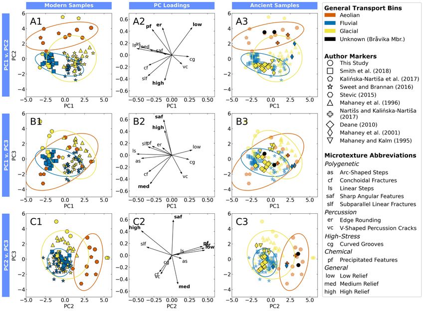
ESSOAr | https://doi.org/10.1002/essoar.10504352.2 | CC_BY_4.0 | First posted online: Sun, 16 May 2021 17:05:40 | This content has not been peer reviewed.

                              Confidential manuscript submitted to the Journal of Sedimentary Research (JSR)

           47      Halverson et al. (2004), there have been three prevailing hypotheses for what depositional

           48      environment the Bråvika could represent:

           49                1) a glaciofluvial outwash plain associated with the overlying Wilsonbreen Formation

           50      (Halverson et al. 2004), which is correlated with the Marinoan “Snowball Earth” pan-glaciation

           51      (Hoffman et al. 2012);

           52                2) an aeolian depositional environment associated with either the glacial conditions of the

           53      Wilsonbreen Formation or the tropical equatorial conditions of the underlying upper Elbobreen

           54      Formation (Halverson 2011), the latter of which is correlated with the Cryogenian interglacial

           55      period (Fairchild et al. 2016); or

           56                3) a tropical fluvial environment associated with the upper Elbobreen Formation

           57      (Hoffman et al. 2012).

           58                To test if our PCA analysis method can constrain the transport histories of ambiguous

           59      ancient sedimentary environments, we transformed two microtextural samples of the Bråvika

           60      Member from Buldrevågen (north-northeast Spitsbergen) into the PCA ordinations. Integrating

           61      the microtextural data with field observations from Buldrevågen, Geerabukta (Ny Friesland), and

           62      Gimleodden (Nordaustlandet), we show that PCA is not only able to distinguish aeolian, fluvial,

           63      and glacial transport modes from each other using microtextural data, but it is also able to help

           64      elucidate the ambiguous transport histories of ancient sediment grains.

           65

           66                                                           MATERIALS

           67                                                          Modern Samples

           68                New Modern Samples. ––– We present five new aeolian samples from the McMurdo

           69      Dry Valleys (Antarctica), Algodones Dunes of California (Cocopah (Kwapa), Kumeyaay, Salt

                                                                                                                                               4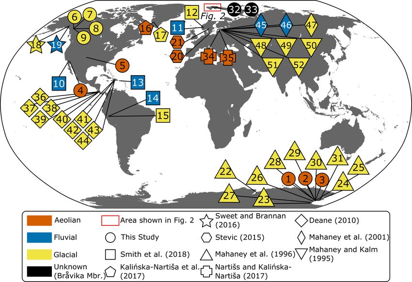
ESSOAr | https://doi.org/10.1002/essoar.10504352.2 | CC_BY_4.0 | First posted online: Sun, 16 May 2021 17:05:40 | This content has not been peer reviewed.

                              Confidential manuscript submitted to the Journal of Sedimentary Research (JSR)

                   Figure 1. Global map of all samples analyzed in this study. The number in each marker
                   corresponds to the sample group number in Tables 1 and 2.

           70      River Pima-Maricopa (O’odham-Piipaash), and Quechan (Kwatsáan) territory), and Waynoka

           71      Dunes of Oklahoma (Comanche (Numunuu), Keechi (Ki:che:ss), Kiowa ([Gáui[dòñ:gyà), Osage

           72      (Wahzhazhe), Tawakoni (Tawá:kharih), Waco (Wí:koʔ), and Wichita (Kirikirʔi:s) territory), as

           73      well as four new glacial samples from the Llewellyn Glacier in British Columbia on Taku River

           74      Tlingit (Lingít) territory (Fig. 1; Table 1). Each of these samples are briefly described in the

           75      following paragraphs, and more detailed descriptions can be found in the Supplementary

           76      Material.

           77                Of the five aeolian samples, three are sourced from perennially ice-covered lakes in the

           78      McMurdo Dry Valleys: one from Lake Fryxell (documented in Jungblut et al. 2016), one from

                                                                                                                                               5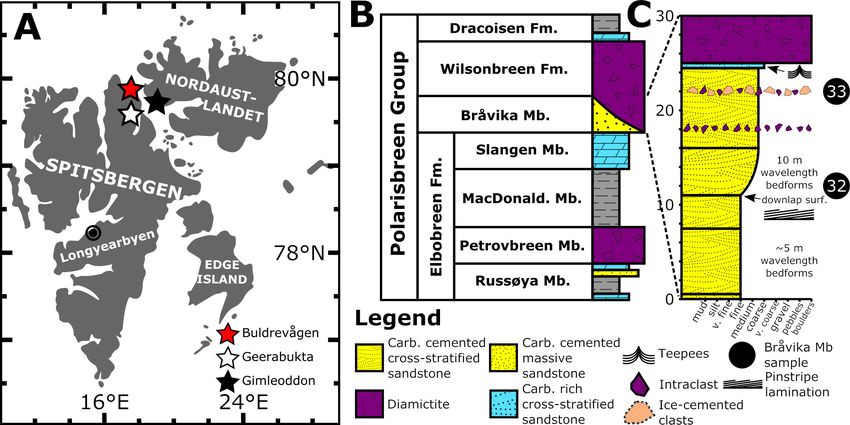
ESSOAr | https://doi.org/10.1002/essoar.10504352.2 | CC_BY_4.0 | First posted online: Sun, 16 May 2021 17:05:40 | This content has not been peer reviewed.

                                Confidential manuscript submitted to the Journal of Sedimentary Research (JSR)

                   Table 1. List of the samples from modern depositional environments considered in this study.
                   Each group of samples is assigned a number for later reference in Figures 1 and 5 (Column #).
                   Column S indicates the number of samples in each sample group, and column N indicates the
                   number of quartz grains in each sample group.

                       Study        #                   Sample Location                      Transport   S     N            GPS Point
                                    1   Lake Fryxell, McMurdo Dry Valleys, Antarctica        Aeolian     1    31    77°36'48"S, 163°06'40"E
                                    2    Lake Joyce, McMurdo Dry Valleys, Antarctica         Aeolian     1    34    77°43'11"S, 161°36'25"E
                                    3    Lake Vanda, McMurdo Dry Valleys, Antarctica         Aeolian     1    30    77°31'38"S, 161°36'24"E
                                    4          Algodones Dunes, California, U.S.             Aeolian     1    44    33°08'57"N, 115°18'48"W
                    This Study      5           Waynoka Dunes, Oklahoma, U.S.                Aeolian     1    48    36°33'35"N, 98°53'56"W
                                    6       Llewellyn Glacier, B.C. (JIF19-C26-01)            Glacial    1    31    59°00'49"N, 134°07'15"W
                                    7       Llewellyn Glacier, B.C. (JIF19-C26-02)            Glacial    1    39    59°00'48"N, 134°07'13"W
                                    8       Llewellyn Glacier, B.C. (JIF19-C26-03)            Glacial    1    36    59°00'48"N, 134°07'13"W
                                    9       Llewellyn Glacier, B.C. (JIF19-C26-04)            Glacial    1    40    59°00'50"N, 134°07'14"W
                                   10        Anza-Borrego Desert, California, U.S.            Fluvial    5    250   32°54'00"N, 116°16'00"W
                                   11         Auster and Storelvi Rivers, Norway              Fluvial    7    346    61°32'00"N, 06°57'00"E
                    Smith et al. 12            Austerdal Glacier Moraine, Norway              Glacial    1    50     61°32'00"N, 06°57'00"E
                      (2018)     13                Rio Guayanés, Puerto Rico                  Fluvial    6    297   18°03'00"N, 65°54'00"W
                                   14                    Rio Parón, Peru                      Fluvial    5    250    09°00'00"S, 77°42'00"W
                                   15        Moraine Proximal to Lake Parón, Peru             Glacial    1    48     09°00'00"S, 77°42'00"W
                     Kalińska-                     Russell Glacier, Greenland
                                   16                                                        Aeolian     3    60    67°05'00"N, 50°20'00"W
                     Nartiša et                        (CE1, CE2, CE8)
                     al. (2017)    17       Russell Glacier, Greenland (CE12, CE13)           Glacial    2    40    67°07'00"N, 50°05'00"W
                                          Chitina Glacier Moraine to 12 km Past Tana
                     Sweet and     18                                                         Glacial    22   626   61°05'44"N, 142°11'03"W
                                        River Confluence, Alaska, U.S. (CR-1 to CR-23)
                      Brannan
                                        12 km Past Tana River Confluence to the Copper
                      (2016)       19                                                         Fluvial    18   450   61°21'42"N, 143°46'34"W
                                             River, Alaska, U.S. (CR-24 to CR-41)
                       Stevic      20       Coastal Sand Dune, Vittskövle, Sweden            Aeolian     1    15     55°51'56"N, 14°10'02"E
                       (2015)      21     Inland Sand Dune, Brattforsheden, Sweden           Aeolian     1    15     59°36'26"N, 13°53'03"E
                                   22   Lichen Valley, Vestfold Hills, Antarctica (Site A)    Glacial    1    25     68°28'53"S, 78°10'24"E
                                        Ackerman Ridge, Scott Glacier area, Antarctica
                                   23                                                         Glacial    1    25    85°45'00"S, 153°00'00"W
                                                        (Sites B – C)
                                        Southern Inexpressible Island, Antarctica (Site
                                   24                                                         Glacial    1    25    74°54'00"S, 163°39'00"E
                                                              D)
                                            Taylor Glacier, McMurdo Dry Valleys,
                                   25                                                         Glacial    1    25    77°44'00"S, 162°10'00"E
                                                     Antarctica (Site E)
                    Mahaney et     26        Hatherton Glacier, Antarctica (Site F)           Glacial    1    25    79°55'00"S, 157°35'00"E
                    al. (1996)
                                   27       Roberts Massif, Antarctica (Sites G – H)          Glacial    2    50    85°32'00"S, 177°05'00"W
                                   28          Barwick Valley, Antarctica (Site I)            Glacial    1    25    77°23'24"S, 161°02'18"E
                                   29        Cambridge Glacier, Antarctica (Site J)           Glacial    1    25    76°57'00"S, 160°31'00"E
                                        Southern Inexpressible Island, Antarctica (Site
                                   30                                                         Glacial    1    25    75°38'00"S, 161°05'00"E
                                                              D)
                                        Luther Peak Basin, Edisto Inlet, Antarctica (Site
                                   31                                                         Glacial    1    25    72°22'00"S, 169°50'00"E
                                                              L)

                                                                                                                                               6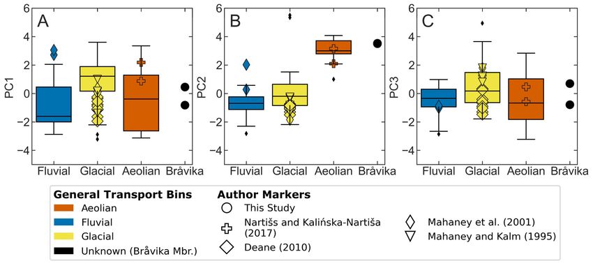
ESSOAr | https://doi.org/10.1002/essoar.10504352.2 | CC_BY_4.0 | First posted online: Sun, 16 May 2021 17:05:40 | This content has not been peer reviewed.

                              Confidential manuscript submitted to the Journal of Sedimentary Research (JSR)

           79      Lake Joyce (documented in Mackey et al. 2015) and one from Lake Vanda (documented in

           80      Mackey et al. 2017). The bulk of coarse-grained sedimentation under the ice cover of these lakes

           81      is wind-blown quartz- and feldspar-rich sand that melts through the ice and is deposited within

           82      layers of microbial mats on the lake floor (Gumbley 1975; Green et al. 2004; Shacat et al. 2004;

           83      Jungblut et al. 2016). The lakes’ lack of wind-driven turbulence (Spigel and Priscu 1998) and

           84      neutral to high pH (Green et al. 2004; Shacat et al. 2004; Jungblut et al. 2016) suggest that these

           85      aeolian grains are negligibly overprinted by lacustrine transport or acidification processes after

           86      they melt through the ice.

           87                The remaining two aeolian samples are from the Algodones Dunes and the Waynoka

           88      Dunes (both documented by Adams 2018; Adams and Soreghan 2020). Both dunefields are

           89      sourced from fluvial deposits (Winspear and Pye 1995; Lepper and Scott 2005) and have been

           90      active since the late Holocene (Stokes et al. 1997; Lepper and Scott 2005). Given that aeolian

           91      transport over short distances and timeframes rapidly imprints aeolian microtextures on quartz

           92      grains (Costa et al. 2013), we expect there to be negligible fluvial overprinting on these samples.

           93                The four glacial samples from the Llewellyn Glacier on the Juneau Icefield were

           94      collected from lateral glacial moraines (JIF19-C26-02 and JIF19-C26-03) and an ephemeral

           95      glaciofluvial melt stream 10 m downstream from a separated branch of ice from the Llewellyn

           96      Glacier (JIF19-C26-01 and JIF19-C26-04; Fig. S1). Because many kilometers of fluvial transport

           97      are needed to create a fluvial microtextural overprint on glacial sediment (Pippin 2016; Sweet

           98      and Brannan 2016; Křížek et al. 2017), samples JIF19-C26-01 and JIF19-C26-04 are more

           99      representative of a glacial setting than a fluvial setting.

         100                 Modern Literature Samples. ––– Previously published aeolian, fluvial, and glacial

         101       samples comprise the remainder of modern samples considered in this study (Fig. 1; Table 1).

                                                                                                                                               7
ESSOAr | https://doi.org/10.1002/essoar.10504352.2 | CC_BY_4.0 | First posted online: Sun, 16 May 2021 17:05:40 | This content has not been peer reviewed.
Confidential manuscript submitted to the Journal of Sedimentary Research (JSR)
102 We selected 5 studies to use in this modern dataset: Mahaney et al. (1996), Stevic (2015), Sweet
103 and Brannan (2016), Kalińska-Nartiša et al. (2017), and Smith et al. (2018).
104 Mahaney et al. (1996) analyzed 11 glacial samples distributed around the Antarctic
105 continent. Stevic (2015) analyzed two aeolian samples, one from a coastal dune in Vittskövle,
106 Sweden and another from an inland sand dune near Brattforsheden, Sweden. Sweet and Brannan
107 (2016) investigated the microtextural transition from glacially-dominated samples to fluvially-
108 dominated ones using 46 samples of sand collected along a transect from the Chitina Glacier to
109 the Copper River in Alaska. For the purposes of sorting these samples into glacial and fluvial
110 bins, we use Sweet and Brannan's (2016) 5-point averaged fluvial-glacial (F/G) microtextural
111 ratio. Samples with a 5-point averaged F/G > 1 are classified as fluvial samples and samples with
112 a 5-point averaged F/G < 1 are classified as glacial. Kalińska-Nartiša et al. (2017) analyzed three
113 aeolian samples and two glacial samples from the Russell Glacier in southwest Greenland.
114 Finally, Smith et al. (2018) analyzed 25 fluvial and glacial samples from the Anza-Borrego
115 Desert in California, the Auster and Storelvi Rivers in Norway, the Rio Guayanés in Puerto Rico,
116 and the Rio Parón in Peru. Because Smith et al. (2018) saw no significant change in percussion
117 features along each of the river transects—even in glaciofluvial settings—the fluvial samples in
118 Smith et al. (2018) are defined as those collected along river transects and the glacial samples
119 are defined as those collected at moraines.
120
121 Ancient Samples
122 Cryogenian Bråvika Member, Svalbard, Norway. ––– We analyzed two samples of
123 the Bråvika Member from a site at Buldrevågen in north-northeast Spitsbergen (Fig. 2), one at 12
124 m and another at 22 m above the base of the Bråvika Member. We will present field observations
8ESSOAr | https://doi.org/10.1002/essoar.10504352.2 | CC_BY_4.0 | First posted online: Sun, 16 May 2021 17:05:40 | This content has not been peer reviewed.
Confidential manuscript submitted to the Journal of Sedimentary Research (JSR)
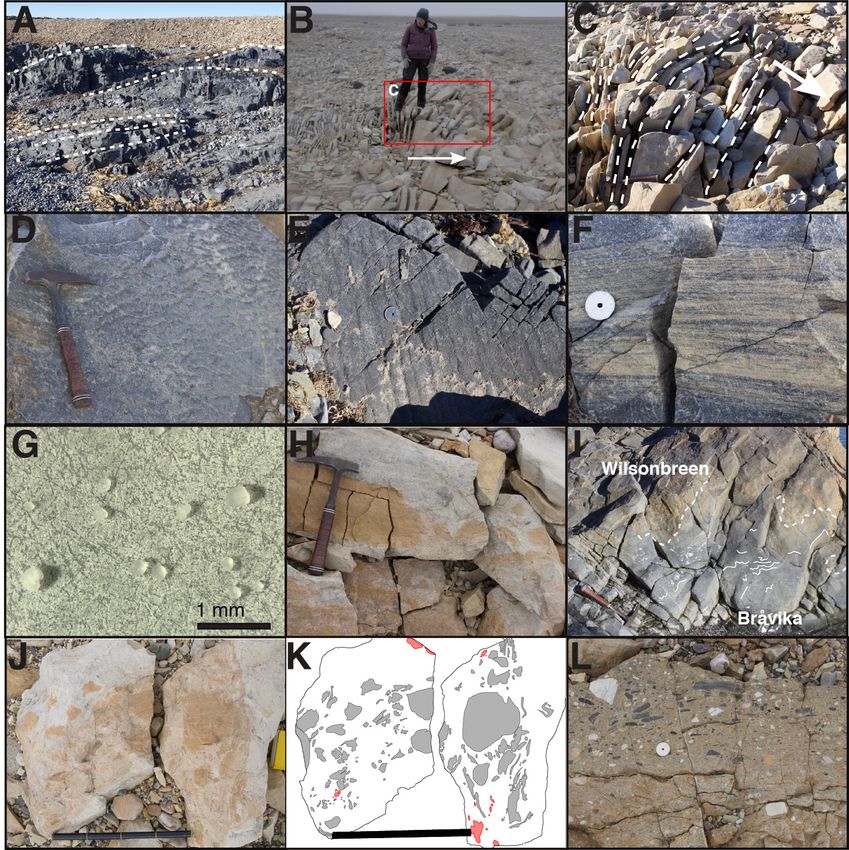
Figure 2. Geologic context and stratigraphy of the Cryogenian Bråvika Member in Svalbard. A)
Map of the Svalbard archipelago. Each star indicates a site observed in this study: Buldrevågen
(red), Geerabukta (white), and Gimleoddon (black). B) Generalized stratigraphic nomenclature
for the Cryogenian Polarisbreen Group in Svalbard after Halverson et al. (2018). As shown here,
the Bråvika Member is assigned to neither the Wilsonbreen nor the Elbobreen formations, as its
assignment is a key question explored in this study. The Petrovbreen Member is correlated with
the Sturtian pan-glaciation and the Wilsonbreen Formation is correlated with the Marinoan pan-
glaciation (Hoffman et al. 2012). The MacDonaldryggen and Slangen members are correlated
with the Cryogenian interglacial (Fairchild et al. 2016). C) Stratigraphic column of the Bråvika
Member at Buldrevågen. The black circles indicate where samples 32 (J1701-156) and 33
(J1701-166) were collected for microtextural analysis.
125 of the Bråvika Member from outcrops in Buldrevågen, Geerabukta (Ny Friesland), and
126 Gimleodden (Nordaustlandet) as context for the microtextural samples.
127 The Cryogenian Bråvika Member is a northward-thickening and coarsening-upward
128 wedge of quartz arenite with lenses and beds of dolomite that outcrop in northeastern Svalbard,
129 Norway (Halverson et al. 2004). The Bråvika Member is situated between two units that are
130 interpreted to represent different Cryogenian climate states (Fig. 2). The underlying siltstone and
131 dolomite of the upper Elbobreen Formation (MacDonaldryggen and Slangen Members) are
9ESSOAr | https://doi.org/10.1002/essoar.10504352.2 | CC_BY_4.0 | First posted online: Sun, 16 May 2021 17:05:40 | This content has not been peer reviewed.
Confidential manuscript submitted to the Journal of Sedimentary Research (JSR)
132 correlated with the warm Cryogenian interglacial period (Fairchild et al. 2016), which spanned
133 from the Sturtian deglaciation to the Marinoan glacial initiation. Absolute age constraints on this
134 period are limited, but the Sturtian deglaciation is constrained between >662.7 ± 6.2 Ma (U-Pb
135 SIMS in South China; Yu et al. 2017) to >657.2 ± 2.4 Ma (Re-Os in Southern Australia; Kendall
136 et al. 2006), and the Marinoan glacial onset is constrained between 639.29 ± 0.26/0.31/0.75 Ma (U-Pb CA-ID-TIMS in
138 Congo; Prave et al. 2016). The overlying glacial diamictites of the Wilsonbreen Formation share
139 a reciprocal thickness relationship with the Bråvika Member and are correlated with the
140 Marinoan glaciation (Hoffman et al. 2012), which ended between 636.41 ± 0.45 Ma (U-Pb CA-
141 ID-TIMS in Southern Australia; Calver et al. 2013) and 635.2 ± 0.6 Ma (U-Pb zircon in South
142 China; Condon et al. 2005).
143 Ancient Literature Samples. ––– In addition to the two Bråvika Member samples, we
144 compiled a set of ancient aeolian, fluvial, and glacial microtextural samples from 4 studies:
145 Mahaney and Kalm (1995), Mahaney et al. (2001), Deane (2010), and Nartišs and Kalińska-
146 Nartiša (2017) (Fig. 1; Table 2).
147 Mahaney and Kalm (1995) analyzed 23 glacial samples from the Pleistocene Dainava,
148 Ugandi, Varduva, and Latvia Tills in Estonia. Mahaney et al. (2001), following Mahaney and
149 Kalm (2000), used quantitative microtextural analysis and Eucledian distances to characterize 29
150 Pleistocene glacial samples, 3 Pleistocene glaciofluvial samples, and 21 Middle Devonian fluvial
151 samples from Estonia. All of these samples were previously collected and analyzed in Mahaney
152 and Kalm (2000). Deane (2010) compared 9 Last Glacial Maximum (LGM) glaciogenic samples
153 from Costa Rica with 9 potentially-glaciogenic samples from the Dominican Republic and found
154 that the two sample sets were statistically indistinguishable, supporting a glaciogenic history for
10ESSOAr | https://doi.org/10.1002/essoar.10504352.2 | CC_BY_4.0 | First posted online: Sun, 16 May 2021 17:05:40 | This content has not been peer reviewed.
Confidential manuscript submitted to the Journal of Sedimentary Research (JSR)
Table 2. List of the samples from ancient depositional environments considered in this study.
Each group of samples is assigned a number for reference in Figures 1, 2, and 6 (Column #).
Column S indicates the number of samples in each sample group, and column N indicates the
number of quartz grains in each sample group.
Study # Sample Transport S N GPS Point Geologic Period
Bråvika Mbr. – Buldrevågen
32 Unknown 1 39 79°59'29"N, 17°31'20"E
(J1701-156)
This Study Cryogenian
Bråvika Mbr. – Buldrevågen
33 Unknown 1 40 79°59'29"N, 17°31'20"E
(J1701-166)
Nartišs and Middle Gauja Lowland,
34 Aeolian 1 16 57°30'00"N, 26°00'00"E
Kalińska- Latvia (Mielupīte 1.3)
Pleistocene
Nartiša Middle Gauja Lowland,
(2017) 35 Aeolian 1 18 57°30'00"N, 26°00'00"E
Latvia (Mielupīte 1.7)
36 Till, Costa Rica (Sample 2) Glacial 1 300 09°29'35"N, 83°29'07"W
37 Till, Costa Rica (Sample 3) Glacial 1 100 09°29'35"N, 83°29'07"W
38 Till, Costa Rica (Sample 4) Glacial 1 100 09°29'35"N, 83°29'07"W
39 Till, Costa Rica (Sample 5) Glacial 1 100 09°29'35"N, 83°29'07"W
40 Till, Costa Rica (Sample 8) Glacial 1 100 09°29'35"N, 83°29'07"W
Deane Till, Dominican Republic
41 Glacial 1 100 19°02'01"N, 71°04'22"W Pleistocene
(2010) (Sample 10)
Till, Dominican Republic
42 Glacial 1 100 19°01'60"N, 71°04'26"W
(Sample 11)
Till, Dominican Republic
43 Glacial 1 100 19°02'07"N, 71°04'38"W
(Sample 17)
Till, Dominican Republic
44 Glacial 1 100 19°01'39"N, 71°02'30"W
(Sample 18)
Arküla Stage Sandstone,
45 Fluvial 21 420 58°15'00"N, 26°30'00"E Middle Devonian
Mahaney et Estonia
al. (2001) 46 Glaciofluvial Sand, Estonia Fluvial 3 60 58°15'00"N, 26°30'00"E
Pleistocene
47 Till, Estonia Glacial 29 580 58°15'00"N, 26°30'00"E
48 Latvia Till, Estonia Glacial 5 100 58°13'28"N, 26°25'16"E
Mahaney 49 Varduva Till, Estonia Glacial 5 100 58°13'28"N, 26°25'16"E
and Kalm 50 Upper Ugandi Till, Estonia Glacial 5 100 58°13'28"N, 26°25'16"E Pleistocene
(1995) 51 Lower Ugandi Till, Estonia Glacial 5 100 58°13'28"N, 26°25'16"E
52 Upper Dainava Till, Estonia Glacial 3 60 58°13'28"N, 26°25'16"E
155 the samples from the Dominican Republic. In our study, we include samples from Deane (2010)
156 that were collected directly from known or hypothesized glacial diamicts and moraines in Costa
157 Rica and the Dominican Republic; we did not include samples from glaciolacustrine
158 environments and debris-flows. Nartišs and Kalińska-Nartiša (2017) analyzed two aeolian
11ESSOAr | https://doi.org/10.1002/essoar.10504352.2 | CC_BY_4.0 | First posted online: Sun, 16 May 2021 17:05:40 | This content has not been peer reviewed.
Confidential manuscript submitted to the Journal of Sedimentary Research (JSR)
159 samples from periglacial aeolian dunes associated with the retreat of the Fennoscandian ice sheet
160 after the LGM in Latvia.
161
162 METHODS
163 Field Work and Sample Collecting
164 Samples analyzed for the first time in this study were collected over multiple field
165 seasons using a variety of methods. The samples from the McMurdo Dry Valleys were originally
166 collected as microbial mats using the methods described in Mackey et al. (2015), Jungblut et al.
167 (2016), and Mackey et al. (2017). Samples from the Algodones Dunes and Waynoka Dunes were
168 collected using the methods described in Adams and Soreghan (2020). On the Juneau Icefield,
169 four sand samples of ~50 g each were collected in August 2019 from glacial moraines and an
170 ephemeral glaciofluvial melt stream on the Llewellyn Glacier (Camp 26) nunatak. Field work on
171 the Bråvika Member in Buldrevågen, Geerabukta, and Gimleodden was performed in 2017.
172
173 Microtextural Sample Disaggregation and SEM Preparation
174 Most samples collected for this study were unconsolidated sediment, but consolidated
175 samples were disaggregated before analysis. Both dolomite-cemented Bråvika Member samples
176 from Svalbard were disaggregated using 1N hydrochloric acid (HCl) at 50°C for 24 hours. Sand
177 samples from Lake Joyce, Lake Fryxell, and Lake Vanda were disaggregated from the microbial
178 mats using 30% hydrogen peroxide (H2O2) solution at 50°C for 24 hours to remove organics and
179 1N HCl at 50°C for 24 hours to remove carbonate.
180 All of the samples were then prepared for blind microtextural analysis in the style of
181 Smith et al. (2018). Samples were distributed into vials and given unique codes unknown to the
12ESSOAr | https://doi.org/10.1002/essoar.10504352.2 | CC_BY_4.0 | First posted online: Sun, 16 May 2021 17:05:40 | This content has not been peer reviewed.
Confidential manuscript submitted to the Journal of Sedimentary Research (JSR)
182 primary researcher. These blinded conditions were maintained until after each sample’s
183 microtextural data were collected.
184 After sample randomization, each sample was gently wet sieved into a 125 µm – 1 mm
185 grain size fraction and dried in an oven. After drying, the samples were treated with 30% H2O2
186 solution at 50°C for 24 hours to remove organics. Samples were then treated with 1N HCl
187 solution for 24 hours at 50°C to remove any remaining carbonate coatings. Neither H2O2 nor
188 low-concentration HCl at these temperatures and time frames affects quartz microtextures (Pye
189 1983; Keiser et al. 2015; Smith et al. 2018).
190 Samples were then treated using the citrate-bicarbonate-dithionite (CBD) method
191 (Janitsky 1986) to remove iron-oxide and manganese-oxide coatings. Between all chemical
192 treatments, the samples were thoroughly rinsed and dried. These samples were not sonicated to
193 prevent artificially inducing microtextures (Porter 1962).
194 Following these treatments, 50 grains that appeared to be quartz (e.g. translucent, no
195 obvious cleavage, etc.) were randomly selected from each sample for microtextural analysis
196 using a reflected-light microscope. The selected grains were mounted on an aluminum SEM stub
197 with double-sided carbon tape in a 10x5 grid and then coated with a 5 nm thick platinum-
198 palladium alloy (Pt/Pd; 80/20) sputter coating to prevent charging under the SEM. Although a
199 gold (Au) or gold-palladium alloy (Au/Pd) coating is frequently used for SEM samples (Vos et
200 al. 2014), Pt/Pd is a better alternative to Au coatings because Pt/Pd coatings have a smaller grain
201 size that allows for higher-resolution analysis (5-10 nm Au vs. 4-8 nm Au/Pd vs. 2-3 nm Pt/Pd;
202 Goldstein et al. 1992).
203
204 SEM Imaging and Analysis
13ESSOAr | https://doi.org/10.1002/essoar.10504352.2 | CC_BY_4.0 | First posted online: Sun, 16 May 2021 17:05:40 | This content has not been peer reviewed.
Confidential manuscript submitted to the Journal of Sedimentary Research (JSR)
205 All grains in each sample were photographed at a 30° tilt on a Zeiss FESEM Supra55VP
206 using a secondary electron (SE2) detector at 20 kV EHT. Viewing the grains at a 30° angle helps
207 to identify smaller microtextures that are difficult to identify at a 0° angle (Margolis and Krinsley
208 1971). During imaging, energy-dispersive spectroscopy (EDS) was used to confirm the
209 composition of each quartz grain.
210 After imaging, each quartz grain was analyzed for the presence or absence of 20
211 microtextures (Fig. 3) according to the methods of Mahaney et al. (2001) and Mahaney (2002).
212 The microtextures are grouped into five bins as defined by Sweet and Soreghan (2010) that
213 differentiate features by formation process: polygenetic, percussion, high-stress, chemical, and
214 grain relief. The following formation descriptions are from Sweet and Soreghan (2010).
215 Polygenetic features are formed through a variety of processes. Percussion features are formed
216 via grain saltation. High-stress features are formed when grains are subjected to high shear
217 stresses. Chemical features are formed via silica dissolution or precipitation. Grain relief refers to
218 the difference between the high and low points on the grain surface.
219 Grains with extreme diagenetic overprint (e.g. ≥ ~90% estimated coverage of diagenetic
220 overprint; Fig. S2) were removed from the sample dataset. The probability of occurrence for
221 each microtexture pm was calculated by dividing the sum of the counts for a given microtexture
222 by the total number of grains in the sample (Smith et al. 2018).
223 Previous microtextural studies have used a range of sample sizes, from less than 20
224 grains per sample (Krinsley and Funnell 1965; Coch and Krinsley 1971; Blackwelder and Pilkey
225 1972) to 100 grains or more per sample (Vincent 1976; Setlow 1978; Deane 2010). This study
226 analyzed ≤ 50 grains per sample as a midpoint between these. However, non-quartz grains and
227 diagenetically overprinted grains were removed from the sample dataset, making 50 grains the
14ESSOAr | https://doi.org/10.1002/essoar.10504352.2 | CC_BY_4.0 | First posted online: Sun, 16 May 2021 17:05:40 | This content has not been peer reviewed.
Confidential manuscript submitted to the Journal of Sedimentary Research (JSR)
Figure 3A. Photos and description of microtextures used in this study. Scale bars are 100 µm unless otherwise noted.
15ESSOAr | https://doi.org/10.1002/essoar.10504352.2 | CC_BY_4.0 | First posted online: Sun, 16 May 2021 17:05:40 | This content has not been peer reviewed.
Confidential manuscript submitted to the Journal of Sedimentary Research (JSR)
Figure 3B. Photos and description of microtextures used in this study. Scale bars are 100 µm unless otherwise noted.
16ESSOAr | https://doi.org/10.1002/essoar.10504352.2 | CC_BY_4.0 | First posted online: Sun, 16 May 2021 17:05:40 | This content has not been peer reviewed.
Confidential manuscript submitted to the Journal of Sedimentary Research (JSR)
228 upper limit for samples in this study. To address this, samples with ≥ 15 eligible quartz grains
229 were considered statistically significant for analysis; samples with < 15 eligible quartz grains
230 were not analyzed. This limit of 15 grains was selected because it is the midpoint of the lower
231 limit recommended sample sizes of Costa et al. (2012), who advocated for a median number of
232 20 grains per sample, and of Vos et al. (2014), who advocated for a lower limit of 10 grains per
233 sample.
234
235 Principal Component Analysis (PCA)
236 We performed PCA on the modern and ancient suites of microtextural data using Scikit-
237 learn 0.21.2 (Pedregosa et al. 2011). This ordination excluded microtextures that were not
238 analyzed by all authors, leaving 12 microtextures that were analyzed by every author in the
239 dataset. These microtextures were arc-shaped steps, conchoidal fractures, linear steps, sharp
240 angular features, subparallel linear fractures, edge rounding, v-shaped percussion cracks, curved
241 grooves, precipitated features, low relief, medium relief, and high relief (Fig. 3; Tables S1–S2).
242 The principal component axes are first derived from the modern suite of microtextural
243 data and then the ancient samples are fitted to these new axes. These axes are shown in three
244 biplots: PC1 vs. PC2; PC1 vs. PC3; and PC2 vs. PC3. In each biplot, 95% confidence ellipses
245 centered at the mean were calculated for each modern transport mode using the methods of
246 Schelp (2019). The broken-stick criterion (Frontier 1976; Jackson 1993; Legendre and Legendre
247 1998; Peres-Neto et al. 2003) was used to determine the significance of the microtextural
248 loadings.
249
250 RESULTS
17ESSOAr | https://doi.org/10.1002/essoar.10504352.2 | CC_BY_4.0 | First posted online: Sun, 16 May 2021 17:05:40 | This content has not been peer reviewed.
Confidential manuscript submitted to the Journal of Sedimentary Research (JSR)
Figure 4. Field observations of the Bråvika Member and related units. All field photographs are
of the Bråvika Member and are credited to K.D. Bergmann unless otherwise noted. A) Annotated
photograph of large-scale bedforms exposed at Gimleodden. Dashed lines trace bedding
surfaces. Hammer for scale. B) Photograph of frost-shattered trough crossbedding at 12 m in
Buldrevågen (Fig. 2C), where the fracture planes are bedding surfaces. Arrow points upsection.
The box highlights the location of C) (Photo credit: A.B. Jost). C) Annotated close-up of trough
crossbedding. The dashed lines trace bedding surfaces and the arrow points upsection. D)
Adhesion ripples on a bedding plane at Geerabukta. E) Potential adhesion ripples on a bedding
plane at Gimleodden. F) Pinstripe lamination at Geerabukta. G) Photomicrograph of frosted
grains from the Bråvika Member at Buldrevågen after dissolution of the dolomite cement with
18ESSOAr | https://doi.org/10.1002/essoar.10504352.2 | CC_BY_4.0 | First posted online: Sun, 16 May 2021 17:05:40 | This content has not been peer reviewed.
Confidential manuscript submitted to the Journal of Sedimentary Research (JSR)
acid (Photo credit: J.N. Reahl). H) Close-up of sand intraclasts with diffuse edges at
Buldrevågen. I) Soft sediment deformation in the upper Bråvika Member under the Wilsonbreen
tillite at Gimleodden, consistent with deformation of unlithified Bråvika sand by overriding ice.
Dashed line marks the diffuse contact between the two units and solid lines trace contorted,
folded beds within the Bråvika Member. Hammer for scale. J) Sandstone intraclasts with diffuse
boundaries and greenish tan, pebbly, coarse sandstone intraclasts at 22 m in Buldrevågen (Fig.
2C). Bar is 40 cm long. K) Line drawing of J at the same scale; sandstone intraclasts are shaded
gray, and greenish tan pebbly, coarse sandstone intraclasts are shaded red. L) The Wilsonbreen
Formation at Buldrevågen, pictured here, has a greenish tan pebbly sandstone matrix.
251 Bråvika Member Field Observations
252 Field observations of the Bråvika Member in Buldrevågen (79°59’29”N, 17°31’20”E),
253 Geerabukta (79°38’06”N, 17°43’48”E), and Gimleodden (79°48’19”N, 18°24’04”E) show
254 evidence of bedforms with 5-10 m wavelength and 1-3 m amplitude, trough cross-bedding,
255 adhesion ripples, pinstripe lamination (at 9 m in Fig. 2C) and grains that are frosted, well-
256 rounded, and well-sorted (Fig. 4A-G). At the Gimleodden site, there is also evidence of soft
257 sediment deformation in the Bråvika Member at the contact with the Wilsonbreen Formation
258 (Fig. 4I). At the Buldrevågen site, the Bråvika Member hosts sandstone intraclasts with diffuse
259 boundaries and no obvious cements at 22 m above the base of the Bråvika Member, as well as
260 pebbly sandstone intraclast conglomerates at 18 m and 22 m (7 m and 3 m below the
261 Wilsonbreen Formation contact, respectively; Figs. 2C, 4J-K). The pebbly sandstone intraclast
262 conglomerate is similar in color to the overlying Wilsonbreen Formation (Fig. 4L).
263
264 Microtextural Dataset Description
265 This microtextural dataset is composed of 113 data points from modern and ancient
266 aeolian, fluvial, and glacial settings. 92 of these data points come from modern settings and 21
267 come from ancient settings. The data are compiled from 10 studies: this study (10% of the total
19ESSOAr | https://doi.org/10.1002/essoar.10504352.2 | CC_BY_4.0 | First posted online: Sun, 16 May 2021 17:05:40 | This content has not been peer reviewed.
Confidential manuscript submitted to the Journal of Sedimentary Research (JSR)
268 datapoints), Smith et al. (2018) (22%), Kalińska-Nartiša et al. (2017) (4%), Nartišs and Kalińska-
269 Nartiša (2017) (2%), Sweet and Brannan (2016) (35%), Stevic (2015) (2%), Deane (2010) (8%),
270 Mahaney et al. (2001) (3%), Mahaney et al. (1996) (10%), and Mahaney and Kalm (1995) (4%).
271 Most data points in this analysis represent a single sample of N grains. The data points from
272 Mahaney and Kalm (1995) and Mahaney et al. (2001) are instead the published averages of
273 larger sets of unavailable raw data from each study.
274 Within the modern samples, 10% of the samples are aeolian, 45% are fluvial, and 45%
275 are glacial. 60% of the modern aeolian samples come from periglacial settings and 73% of the
276 modern fluvial samples come from glaciofluvial settings. All of the modern glacial samples
277 come from active glacial environments. Within the ancient samples, 90% are constrained to
278 particular depositional environments: 10% of the samples are aeolian, 10% are fluvial, and 71%
279 are glacial. The remaining 10% of the ancient samples are from the Cryogenian Bråvika
280 Member, and determining their depositional setting is a goal of this study.
281
282 Probability of Occurrence
283 Modern Samples. ––– Modern aeolian samples are the most likely to have edge
284 rounding (0.90 avg.), precipitated features (0.59 avg.), and low relief (0.31 avg.) compared to
285 modern fluvial and glacial samples, which in turn are more likely to have high relief (0.40 fluvial
286 avg.; 0.36 glacial avg.) and subparallel linear fractures (0.63 fluvial avg.; 0.50 glacial avg.) (Fig.
287 5). These transport modes also share similar probabilities of occurrence for some features.
288 Glacial and aeolian samples share similar probabilities of curved grooves (0.33 glacial avg., 0.27
289 aeolian avg.) compared to fluvial samples. Fluvial and aeolian samples also share similar
290 probabilities of v-shaped percussion cracks (0.45 fluvial avg., 0.48 aeolian avg.) compared to
20ESSOAr | https://doi.org/10.1002/essoar.10504352.2 | CC_BY_4.0 | First posted online: Sun, 16 May 2021 17:05:40 | This content has not been peer reviewed.
Confidential manuscript submitted to the Journal of Sedimentary Research (JSR)
Figure 5. Heatmap of the microtextural probabilities of occurrence from 0 to 1 for each modern
sample group used in the analysis. Samples are binned into aeolian, fluvial, and glacial transport
modes. Refer to Table 1 for sample group numbers and descriptions. Data are averaged for
sample groups that contain more than one sample (S > 1). Refer to Figure 3A and B for
microtextural abbreviations. The average of each transport mode for the modern samples (AVG)
is at the bottom of each bin. Microtextures that were not analyzed within a study are grayed out.
291 glacial samples. The probability of occurrence of arc-shaped steps, conchoidal fractures, linear
292 steps, sharp angular features, and medium relief are not substantially different between the three
293 transport modes.
21ESSOAr | https://doi.org/10.1002/essoar.10504352.2 | CC_BY_4.0 | First posted online: Sun, 16 May 2021 17:05:40 | This content has not been peer reviewed.
Confidential manuscript submitted to the Journal of Sedimentary Research (JSR)
294 Study-specific variations in microtextural probabilities occur within each transport mode.
295 In the aeolian transport mode, samples from Stevic (2015) (samples 20–21; Table 1) are more
296 likely to have curved grooves (0.80–0.93) compared to other aeolian samples in the dataset
297 (0.13–0.19). The fluvial grains from Sweet and Brannan (2016) (sample 19) are more likely to
298 have v-shaped percussion cracks (0.82) compared to the remaining fluvial samples from Smith et
299 al. (2018) (0.15–0.40). Glacial grains from this study (samples 6–9) and Kalińska-Nartiša et al.
300 (2017) (sample 17) have the highest probabilities of edge rounding (0.29–0.91) and precipitated
301 features (0.55–0.88) compared to the remaining glacial samples. The glacial grains from
302 Kalińska-Nartiša et al. (2017) are also the most likely to have low relief (0.68).
303 Ancient Samples. ––– Both samples from the Cryogenian Bråvika Member (samples 32–
304 33; Table 2) have high probabilities of edge rounding (1.00), precipitated features (1.00), and
305 upturned plates (0.85–0.97; Fig. 6). Pleistocene aeolian sand samples from Nartišs and Kalińska-
306 Nartiša (2017) (samples 34–35) have high abundances of edge rounding, dissolution etching, and
307 precipitated features (all categorized as “abundant”; >0.75 probability of occurrence). Grains
308 from the middle Devonian Arküla Stage fluvial sand samples (sample 45) and Pleistocene
309 glaciofluvial sand samples (sample 46) from Estonia (Mahaney et al. 2001) are more likely to
310 have edge rounding (0.56–0.64), v-shaped percussion cracks (0.53–0.61), and low relief (0.35–
311 0.59) compared to grains from the modern fluvial average. The fluvial samples from Mahaney et
312 al. (2001) also have lower probabilities of arc-shaped steps (0.00–0.23), conchoidal fractures
313 (0.06–0.39), linear steps (0.00–0.26), subparallel linear fractures (0.08–0.35), upturned plates
314 (0.00–0.04), and high relief (0.05–0.18) compared to the modern fluvial average. Grains from the
315 Pleistocene tills in Costa Rica and the Dominican Republic (samples 36-44; Deane 2010) are
316 more likely to have subparallel linear fractures (0.86-0.96) and medium relief (0.60-0.76)
22ESSOAr | https://doi.org/10.1002/essoar.10504352.2 | CC_BY_4.0 | First posted online: Sun, 16 May 2021 17:05:40 | This content has not been peer reviewed.
Confidential manuscript submitted to the Journal of Sedimentary Research (JSR)
Figure 6. Heatmap of the microtextural probabilities of occurrence from 0 to 1 for each ancient
sample group used in the analysis. Samples are binned into “unknown” (UNK; Bråvika
Member), aeolian, fluvial, and glacial transport modes. Refer to Table 2 for sample group
numbers and descriptions. Data are averaged for sample groups that contain more than one
sample (S > 1). Refer to Figure 3A and B for microtextural abbreviations. The average of each
transport mode for the modern samples (M. AVG) from Figure 5 is at the bottom of each bin.
Microtextures that were not analyzed within a study are grayed out.
317 compared to the modern glacial average. The Pleistocene tills from Mahaney et al. (2001)
318 (sample 47) and Mahaney and Kalm (1995) (samples 48-52) are broadly comparable to the
319 modern glacial average.
320
321 Principal Component Analysis
322 Within the PCA ordination, the PC1, PC2, and PC3 axes capture about 66% of the
323 variance in the modern dataset (27.01%, 21.33%, and 17.43%, respectively). Along the PC1 axis
23ESSOAr | https://doi.org/10.1002/essoar.10504352.2 | CC_BY_4.0 | First posted online: Sun, 16 May 2021 17:05:40 | This content has not been peer reviewed.
Confidential manuscript submitted to the Journal of Sedimentary Research (JSR)
Figure 7. Boxplots of the modern aeolian, fluvial, and glacial samples along the PC1 (A), PC2
(B), and PC3 (C) axes. The small black diamonds represent modern outliers for each transport
mode. The ancient samples are plotted as individual points over the boxplots.
324 (Figs. 7–8; Table S3), the aeolian, fluvial, and glacial samples are distributed along both sides of
325 the axis with no clear separation. However, the samples are generally separated by study along
326 PC1: the samples from Stevic (2015) and Smith et al. (2018) are distributed between -2.9 and -
327 1.1 and the samples from Mahaney et al. (1996) and Sweet and Brannan (2016) are distributed
328 between -0.2 and 3.5. The samples from this study and Kalińska-Nartiša et al. (2017) are widely
329 distributed on PC1, where the samples from this study are distributed between -3.2 to 3.3 and the
330 Kalińska-Nartiša et al. (2017) samples are distributed between -3.1 and 1.7. The sample
331 separation along PC1 is predominantly driven by the abundance of linear steps and arc-shaped
332 steps, which have the largest (-0.489) and second largest (-0.425) negative loadings along PC1
333 (Table 3). However, neither of these loadings are strongly associated with PC1 according to the
334 broken-stick criterion.
335 Along the PC2 axis, modern aeolian samples are distinctly separated from modern glacial
336 and fluvial samples. This separation between aeolian and fluvial/glacial samples along PC2 is
24ESSOAr | https://doi.org/10.1002/essoar.10504352.2 | CC_BY_4.0 | First posted online: Sun, 16 May 2021 17:05:40 | This content has not been peer reviewed.
Confidential manuscript submitted to the Journal of Sedimentary Research (JSR)
Figure 8. PCA ordination using all 12 microtextures analyzed by all studies. Each row is a biplot
in A) PC1-PC2 space; B) PC1-PC3 space; and C) PC2-PC3 space. Column 1 plots the modern
sample data within each space (this study through Mahaney et al. 1996), Column 2 plots the
microtextural loadings, and Column 3 plots the ancient sample data (this study, Nartišs and
Kalińska-Nartiša 2017 through Mahaney and Kalm 1995) over the existing modern reference
frame. Refer to Table 3 for the loadings in Column 2. Microtextures with significant loadings in
Column 2 are in bold. The ellipses are 95% confidence intervals of each modern transport mode
that are centered at the mean of the transport mode in each coordinate space. The ellipses are
calculated using the methods of Schelp (2019).
337 driven by low relief, edge rounding, and precipitated features in the positive direction (loadings
338 of 0.457, 0.455, and 0.432) and high relief in the negative direction (-0.427), which are all
339 associated with PC2 according to the broken-stick criterion.
340 Along the PC3 axis, the three transport modes are distributed along both sides of the axis
341 with no clear separation, similar to the distribution along PC1. However, unlike the distribution
25ESSOAr | https://doi.org/10.1002/essoar.10504352.2 | CC_BY_4.0 | First posted online: Sun, 16 May 2021 17:05:40 | This content has not been peer reviewed.
Confidential manuscript submitted to the Journal of Sedimentary Research (JSR)
Table 3. Ranked loadings and squared loadings of microtextures from the PCA ordination (Fig.
8). Refer to Figure 3A and B for microtexture abbreviations. The microtextures in bold have
squared loadings that are greater than the expected value of their associated principal component
according to the broken-stick criterion (Frontier 1976; Jackson 1993; Legendre and Legendre
1998; Peres-Neto et al. 2003).
PC1 PC2 PC3
Expected PC Value: 0.259 Expected PC Value: 0.175 Expected PC Value: 0.134
2 2
Microtexture Loading Loading Microtexture Loading Loading Microtexture Loading Loading 2
low 0.286 0.082 low 0.457 0.209 saf 0.592 0.351
cg 0.239 0.057 er 0.455 0.207 high 0.411 0.169
vc 0.141 0.020 pf 0.432 0.186 pf 0.153 0.023
high -0.104 0.011 as 0.139 0.019 slf 0.135 0.018
saf -0.114 0.013 ls 0.112 0.013 er 0.126 0.016
er -0.128 0.017 med 0.090 0.008 low 0.089 0.008
pf -0.272 0.074 saf 0.018 0.000 ls 0.019 0.000
med -0.300 0.090 cg -0.028 0.001 as -0.055 0.003
cf -0.324 0.105 vc -0.153 0.023 cg -0.071 0.005
slf -0.335 0.112 cf -0.168 0.028 cf -0.279 0.078
as -0.425 0.181 slf -0.350 0.123 vc -0.312 0.097
ls -0.489 0.239 high -0.427 0.182 med -0.482 0.232
342 along PC1, the samples are not as distinctly separated by study. The significant microtextures
343 along PC3 are sharp angular features and high relief in the positive direction (0.592 and 0.411),
344 and medium relief in the negative direction (-0.482). All of these microtextures are associated
345 with PC3 according to the broken-stick criterion.
346 Along each principal component axis, at least 89% of the ancient aeolian, fluvial, and
347 glacial samples plot within the upper and lower adjacent values of the boxplot of their modern
348 counterparts: 89% on PC1, 95% on PC2, and 100% on PC3 (Fig. 7). In each biplot (Fig. 8), at
349 least 74% of these ancient samples plot within the 95% confidence ellipses of their modern
350 counterparts: 89% in the PC1-PC2 biplot (A3), 74% in the PC1-PC3 biplot (B3), and 95% in the
351 PC2-PC3 biplot (C3). The median of the percent agreement between the ancient samples and
352 their modern counterparts is 92%.
26ESSOAr | https://doi.org/10.1002/essoar.10504352.2 | CC_BY_4.0 | First posted online: Sun, 16 May 2021 17:05:40 | This content has not been peer reviewed.
Confidential manuscript submitted to the Journal of Sedimentary Research (JSR)
353 The 92% median agreement between the modern and ancient samples demonstrates that
354 PCA of modern and ancient samples provides a valid framework for interpreting the fingerprint
355 of depositional environments in ancient samples with ambiguous depositional histories. In this
356 ordination, the two Bråvika Member samples with ambiguous depositional histories consistently
357 plot within the upper and lower adjacent values of the modern aeolian samples in each principal
358 component axis (Fig. 7) and the 95% confidence ellipses of the modern aeolian samples in each
359 biplot (Fig. 8). This placement suggests that the Bråvika Member samples analyzed in this study
360 have an aeolian origin.
361
362 DISCUSSION
363 Interpreting the PCA Ordination
364 PC1 separates the modern samples by author and accounts for the most variance in the
365 dataset (27.01%), indicating that author-specific microtextural variance is the largest individual
366 source of variance in the modern dataset. This result is consistent with the observation that SEM
367 operator variance exerts significant influence on the probabilities of occurrence of individual
368 microtextures (Culver et al. 1983). However, as Culver et al. (1983) observed using canonical
369 variate analysis, author variance is overall negligible in determining a sample’s depositional
370 environment: the combined variance of PC2 and PC3 accounts for over a third of the variance in
371 the modern dataset (21.33% and 17.43%, respectively). The PC2 axis separates the samples into
372 aeolian and fluvial/glacial transport modes, and the PC3 axis separates the samples neither by
373 transport mode nor by study (Fig. 8).
374
375 Which Microtextures Distinguish Transport Modes?
27ESSOAr | https://doi.org/10.1002/essoar.10504352.2 | CC_BY_4.0 | First posted online: Sun, 16 May 2021 17:05:40 | This content has not been peer reviewed.
Confidential manuscript submitted to the Journal of Sedimentary Research (JSR)
376 Aeolian sediment is defined by high probabilities of low relief, edge rounding, and
377 precipitated features, and fluvial and glacial sediments are defined by high probabilities of high
378 relief and subparallel linear fractures. The modern (Fig. 5) and ancient (Fig. 6) heatmaps show
379 that aeolian samples have the highest probabilities of low relief, edge rounding, and precipitated
380 features, and fluvial and glacial samples have the highest probabilities of high relief and
381 subparallel linear fractures. PC2 also separates the aeolian samples from the fluvial and glacial
382 samples using low relief, edge rounding, and precipitated features in the positive (aeolian)
383 direction and high relief in the negative (fluvial/glacial) direction (Fig. 8; Table 3). These
384 findings are consistent with previous observations of these microtextures: low relief, edge
385 rounding, and precipitated features have all previously been associated with windblown sediment
386 (Nieter and Krinsley 1976; Lindé and Mycielska-Dowgiałło 1980; Krinsley and Trusty 1985;
387 Mahaney 2002; Vos et al. 2014); high relief can occur on both fluvial and glacial sediments
388 (Mahaney 2002; Vos et al. 2014); and subparallel linear fractures are often associated with
389 glacial and glaciofluvial settings, the latter of which makes up 73% of the modern fluvial
390 samples in this study (Mahaney and Kalm 2000; Deane 2010; Immonen 2013; Vos et al. 2014;
391 Woronko 2016).
392 Although fluvial and glacial samples are microtexturally distinct from aeolian samples, it
393 is difficult to disambiguate the fluvial and glacial transport modes from each other in this dataset.
394 Features that are typically associated with glacial environments, such as arc-shaped steps,
395 conchoidal fractures, linear steps, and sharp angular features (Mahaney and Kalm 2000;
396 Mahaney 2002; Immonen 2013; Woronko 2016), had comparable probabilities across all three
397 modern transport modes, indicating that these features are not exclusively associated with glacial
398 environments (Fig. 5). Smith et al. (2018) also observed that arc-shaped steps and linear steps
28ESSOAr | https://doi.org/10.1002/essoar.10504352.2 | CC_BY_4.0 | First posted online: Sun, 16 May 2021 17:05:40 | This content has not been peer reviewed.
Confidential manuscript submitted to the Journal of Sedimentary Research (JSR)
399 may not be indicators of glacial transport. These results are consistent with Sweet and Soreghan
400 (2010)’s classification of these features as polygenetic features that are formed through a variety
401 of transport processes. Subparallel linear fractures are also associated with glacial and
402 glaciofluvial settings (Mahaney and Kalm 2000; Deane 2010; Immonen 2013; Vos et al. 2014;
403 Woronko 2016), but the modern fluvial average for subparallel linear fractures is higher than the
404 glacial average. Although glaciofluvial samples make up 73% of the modern fluvial samples, the
405 non-glacial fluvial samples (samples 10 and 13; Fig. 5) have similar probabilities of subparallel
406 linear fractures compared to glaciofluvial samples (samples 11, 14, and 19), suggesting that
407 subparallel linear fractures may not be an exclusively glacial feature. These results suggest that
408 fluvial and glacial samples may share microtextural similarities, but more studies comparing the
409 microtextural features of non-glacial fluvial, glaciofluvial, and glacial samples are needed to
410 understand the differences between these transport environments.
411 These results highlight the importance of precipitated features as a primary indicator of
412 transport instead of an exclusive product of diagenesis. If precipitated features were only an
413 indicator of post-depositional diagenesis, then the probability of precipitated features should
414 increase with age. However, all of the modern samples have some probability of having
415 precipitated features—particularly the aeolian samples—and the ancient samples do not show a
416 consistent increase in the probability of chemical features as the sediment age increases (Figs. 5–
417 6). Both of these observations point to precipitated features being a primary microtextural
418 feature. Although Sweet and Soreghan (2010) suggested that precipitated features should not be
419 counted because they can form via diagenesis and overprint a sample, our results indicate that
420 these features can also be a primary feature and should not be discounted, even in situations
421 where diagenesis is a concern.
29You can also read