Minimal number of discrete velocities for a flow description and internal structural evolution of a shock wave
←
→
Page content transcription
If your browser does not render page correctly, please read the page content below

Minimal number of discrete velocities for a flow
                                         description and internal structural evolution of a
arXiv:1107.3196v2 [math-ph] 9 Jul 2020

                                                            shock wave
                                                                          Jae Wan Shim
                                         Materials and Life Science Research Division, Korea Institute of
                                                          Science and Technology, and
                                         Major of Nanomaterials Science and Engineering, KIST Campus,
                                                   Korea University of Science and Technology,
                                          5 Hwarang-ro 14-gil, Seongbuk, Seoul 02792, Republic of Korea

                                                                              Abstract
                                                  A fluid flow is described by fictitious particles hopping on homoge-
                                              neously distributed nodes with a given finite set of discrete velocities. We
                                              emphasize that the existence of a fictitious particle having a discrete ve-
                                              locity among the set in a node is given by a probability. We describe
                                              a compressible thermal flow of the level of accuracy of the Navier-Stokes
                                              equation by 25 or 33 discrete velocities for two-dimensional space and per-
                                              form simulations for investigating internal structural evolution of a shock
                                              wave.

                                            Keywords: discrete kinetic theory, internal structural shock wave, Navier-
                                         Stokes equation.

                                         1    Introduction
                                         It seems intuitively correct to describe fluid flows by using fictitious particles
                                         hopping on homogeneously separated nodes with a given finite set of discrete
                                         velocities, however, it is not clear how many discrete velocities are needed for
                                         the motion of the fictitious particles to satisfy a certain level of accuracy with
                                         acceptable stability. This question is clarified by the discrete Boltzmann equa-
                                         tion, which is originally developed from the cellular automata to fluid flows.
                                         Here we show that we can describe a compressible thermal flow of the level of

                                                                                   1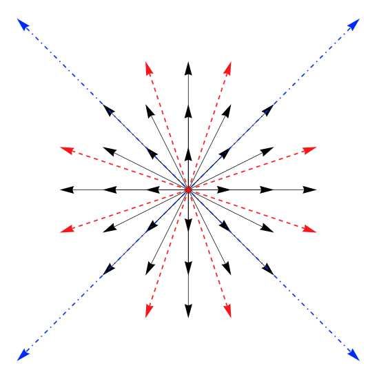
accuracy of the Navier-Stokes equation by 25 or 33 discrete velocities for two-
dimensional space comprised of a square lattice. We look inside the evolution
of shock structure by using the fictitious particles.

2     Rules of collision and movement
The lattice Boltzmann equation [1, 2], originally developed from the cellular au-
tomata [3, 4] to fluid flows, describes a fluid flow by using the notion of fictitious
particles moving their positions and changing their distribution according to a
simple rule
                 fi (x + vi ∆t, t + ∆t) = (1 − ω)fi (x, t) + ωfieq (x, t)                (1)
where fi (x, t) is the density of particles having discrete velocities vi at position
x and at time t, the reference density distribution fieq (x, t) is the density in
equilibrium states settled down from fi (x, t), and ω adjusts viscosity. Because of
the discretized characteristic of the velocity space, fieq (x, t) is not the Maxwell-
Boltzmann distribution itself but can be expressed by weight coefficients wi and
a polynomial approximated from the Maxwell-Boltzmann distribution. We can
recover macroscopic physical properties such as density, velocity, pressure, and
temperature from fi (x, t). To make this particle or lattice-gas method efficient,
it is highly desirable to minimize the number of discrete velocities with keeping
accuracy and stability.
     An important study [5] showed that compressible thermal flows of the level
of accuracy of the Navier-Stokes equation could be recovered by using the lat-
tice Boltzmann equation with 37 discrete velocities in two-dimensional space
comprised of a square lattice and this was confirmed again [6]. However, we can
reduce the minimal number by altering discrete velocities. Here, we present a
33-velocities model having the same order of accuracy to the 37-velocities one.
As described in Fig. 1, the vectors of the 33-velocities model are sparsely and
widely distributed than those of the 37-velocities one. The discrete velocities of
the 33-velocities model vi = (vi,x , vi,y ) is comprised of v1 = (0, 0), v2 = c(1, 0),
v3 = c(2, 0), v4 = c(3, 0), v5 = c(1, 1), v6 = c(2, 2), v7 = c(4, 4), v8 = c(2, 1) and
the other velocities obtained by the symmetry with respect to the x-axis, y-axis,
and y = x where c = 0.819381, so that the discrete velocities satisfy isotropy.
Their corresponding weight coefficients are w1 ≈ 0.161987, w2 ≈ 0.143204,
w3 ≈ 0.00556112, w4 ≈ 0.00113254, w5 ≈ 0.0338840, w6 ≈ 0.0000844799,
w7 ≈ 3.45552 × 10⁻⁶ , w8 ≈ 0.0128169, and for the other velocities obtained by
the symmetry, wi = wj if kvi k = kvj k. For simplicity, we have presented the
approximate values of c and wi with six significant figures instead of the exact
values. Note that this solution can be obtained by the system of equations
                       33
                     X
                              a    b         1+a       1+b
                          wi vi,x vi,y = Γ         Γ           /π
                      i=1
                                              2          2

for (a, b) = (0, 0), (0, 2), (2, 2), (0, 4), (2, 4), (0, 6), (4, 4), (2, 6), and (0, 8) where
Γ is the Gaussian Gamma function [7]. The discretized equilibrium distribution

                                             2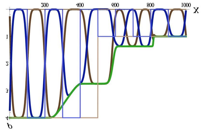
Figure 1: The discrete velocities of the 33-, and 37-velocities models are de-
scribed by the black and the blue (dot-dashed) arrows, and the black and the
red (dashed) arrows, respectively. Note that the zero velocity is omitted.

is obtained by the Hermite expansion of the Maxwell-Boltzmann distribution
[8] as
                                    4
                                   X   1 (n)
                        fieq = ρwi        a · H(n)
                                   n=0
                                       n!
where

         a(0) · H(0) = 1,
         a(1) · H(1) = 2u · vi ,
         a(2) · H(2) = 4(u · vi )2 + 2(θ − 1)(vi2 − 1) − 2u2 ,
         a(3) · H(3) = 4(u · vi ) 2(u · vi )2 − 3u2 + 3(θ − 1)(−2 + vi2 ) ,


         a(4) · H(4) = 16(u · vi )4 − 48(u · vi )2 u2 + 12u4
                     + 24(θ − 1) 2(u · vi )2 (vi2 − 3) + (2 − vi2 )u2


                     + 12(θ − 1)2 (vi4 − 4vi2 + 2),

ρu = vi fi , and ρθ = kvi − ui k2 fi .
      P                  P
   Note that a 25-velocities model for a two-dimensional space is obtained for
the level of accuracy of the Navier-Stokes equation by the tensor product of the
5-velocities model as in [9] by using the coefficients of the Lagrange interpolat-
ing polynomials expressed by the discrete velocities and using moments of the

                                          3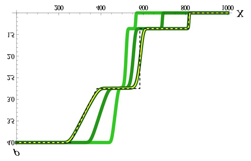
Maxwell-Boltzmann distribution. The shock tube simulation shows relatively
stable and accurate results. This model is less expensive than the 33-velocities
model with respect to the computational cost, however, it is less stable in the
flow regime of high Mach numbers.

3    Internal structural evolution of a shock wave
We illustrate the accuracy and the stability of the 33-velocities model by a shock
tube simulation. A two-dimensional shock tube, whose calculation domain is
comprised of 1000 × 8 nodes, has been simulated by the two models of the 33-
velocities and the 37-velocities with the equilibrium distribution fieq obtained
by the fourth-order Hermite expansion [10]. Initially, the flow is stationary, and
the density and the pressure of the left-half plane are four times higher than
those of the right-half plane, while the temperatures are the same in both sides.
The left and the right boundary conditions are the same to the left and the
right initial conditions, respectively. On the upper and the lower boundaries,
the symmetric conditions are used. The constant ω adjusting viscosity is chosen
as ω = 1. The result of the density distribution has no transversal gradient;
therefore we show the profile with respect to the longitudinal axis in Fig. 2. The
results obtained by the two models are in excellent agreement. The shock front
sharpness of the simulation result is blunt with respect to the analytical solution
of the Riemann problem [11] because of the non-zero viscosity in contrast to the
Riemann problem.
     The simple and easy implantation of the multi-component flows is one of the
advantages of the flow description by the notion of fictitious particles, on which
we just add name tags. We simulate a two-component flow with the previous
simulation setup. However, the domain is divided into 10 vertical strips and we
fill the two components, alternately. The simulation result is shown in Fig. 3.
The inside structure of the shock is well described.

4    Multi-component and complex geometry flow
     simulation
Another advantage of the notion of fictitious particles is that the simulation
method is easily applicable to complex geometry. As an example, the two-
component flow is simulated on a plane having a calculation domain comprised
of 200 × 200 nodes with an arbitrary complex initial condition. The first row of
Fig. 4 shows the initial density distribution of the components A and B. On the
element figures of the first row, the values of density are indicated. The pressure
is the same value to the density. The flow is stationary and the temperature
is uniform at the initial moment. The simulations illustrate the accuracy and
the stability under given conditions. A similar study can be easily done for
three-dimensional space.

                                        4
Figure 2: Comparison of the scaled density ρ obtained by the 33-velocities model
at relative time t′ = 0.2, 0.6, and 1 (from the light green line to the dark), the
37-velocities model at t′ = 1 (yellow), and the analytical solution of the Riemann
problem at t′ = 1 (dashed black).
5Figure 3: Result of the two-component flow simulation. The total density
(green) and each component densities (blue and brown) are drawn t′ = 1. Note
that the thin blue and brown lines show the initial state and the thick lines
show the state after the evolution of time.
6Figure 4: Result of the two-component flow having a geometrically complex
initial condition. The first, the second, and the third rows show the density
distributions at relative time t′ = 0, 0.5, and 1, respectively. On the element
figures of the first row, the values of density are indicated.
75 Conclusion
We have briefly introduced a method for describing a compressible thermal flow
of the level of accuracy of the Navier-Stokes equation by fictitious particles
hopping on homogeneously distributed nodes with a given finite set of discrete
velocities where the existence of a fictitious particle having a discrete velocity
among the set in a node is given by a probability. We have performed sim-
ulations for investigating internal structural evolution of shock waves by the
method which has advantages in dealing with multi-component flows and com-
plex geometry.
Acknowledgement
This work was partially supported by the KIST Institutional Program.
References
[1] Shiyi Chen and Gary D Doolen. Lattice boltzmann method for fluid flows.
Annual review of fluid mechanics, 30(1):329–364, 1998.
[2] Hudong Chen, Satheesh Kandasamy, Steven Orszag, Rick Shock, Sauro
Succi, and Victor Yakhot. Extended boltzmann kinetic equation for tur-
bulent flows. Science, 301(5633):633–636, 2003.
[3] Daniel H Rothman and Stiphane Zaleski. Lattice-gas cellular automata:
simple models of complex hydrodynamics, volume 5. Cambridge University
Press, 2004.
[4] Jae Wan Shim and Renée Gatignol. Robust thermal boundary conditions
applicable to a wall along which temperature varies in lattice-gas cellular
automata. Physical Review E, 81(4):046703, 2010.
[5] Paulo C Philippi, Luiz A Hegele Jr, Luı́s OE Dos Santos, and Rodrigo
Surmas. From the continuous to the lattice boltzmann equation: The dis-
cretization problem and thermal models. Physical Review E, 73(5):056702,
2006.
[6] Xiaowen Shan et al. General solution of lattices for cartesian lattice
bhatanagar-gross-krook models. Physical Review E, 81(3):036702, 2010.
[7] Jae Wan Shim. Multidimensional on-lattice higher-order models in the
thermal lattice boltzmann theory. Physical Review E, 88(5):053310, 2013.
[8] Jae Wan Shim and Renée Gatignol. How to obtain higher-order multivari-
ate hermite expansion of maxwell–boltzmann distribution by using taylor
expansion? Zeitschrift für angewandte Mathematik und Physik, 64(3):473–
482, 2013.
8[9] Jae Wan Shim. Parametric lattice boltzmann method. Journal of Compu-
tational Physics, 338:240–251, 2017.
[10] Harold Grad. Note on n-dimensional hermite polynomials. Communica-
tions on Pure and Applied Mathematics, 2(4):325–330, 1949.
[11] Richard Courant and Kurt Otto Friedrichs. Supersonic flow and shock
waves, volume 21. Springer Science & Business Media, 1999.
9You can also read