The Met Office hourly 4D-Var system, status and plans - ISDA Munich, 07/03/2018 Marco Milan*, Bruce Macpherson, Helen Buttery, Adam Clayton ...
←
→
Page content transcription
If your browser does not render page correctly, please read the page content below

The Met Office
          hourly 4D-Var system,
             status and plans

                              ISDA
                        Munich, 07/03/2018

 Marco Milan*, Bruce Macpherson, Helen
Buttery, Adam Clayton, Gareth Dow, Gordon
  Inverarity, Robert Tubbs, Marek Wlasak
 www.metoffice.gov.uk                        © Crown Copyright 2018 Met Office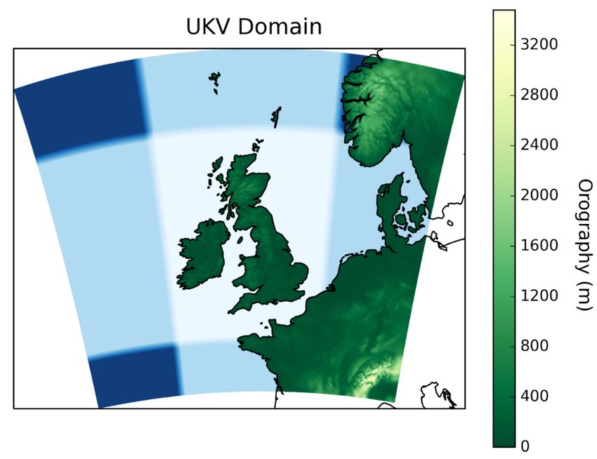
OVERVIEW

• Hourly UKV 4D-Var.
• Observations used.
• Cut-off time and reduction of observations.
• Value of the observations (FSOI).
• Issues in the definition of a background error covariance
  matrix and possible solutions.
• Possible different approach to hourly cycling.

                                      2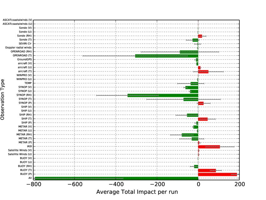
UKV model
• Hourly 4D-Var assimilation method, operational
since July 2017.
• Linear Perturbation Forecast (PF) model and DA,
4.5 km resolution (constant on the whole domain).
• UM model resolution in UK region 1.5km.
Resolution 1.5×4 km resolution along the edges
and 4×4 km at the corners.
• Global boundary conditions 10 km resolution.
• LBC from 00, 06, 12, 18 UTC runs of 10km Global
model
• ‘Age’ of LBC runs lies in range hh-3hrhh-8hr
• Observation cut-off 45 mins.
• Apply varbc to satellite radiances.
3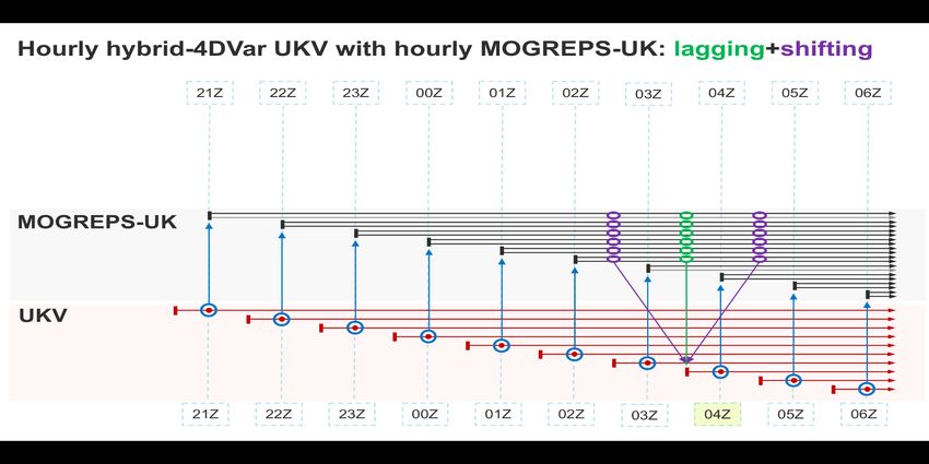
Hourly UKV-4DVar cycle
   T-30’            T+45’
                            OBS cut off T+0            • Cycle for T+0 (e.g. 01 UTC)
                                                          • Assimilation window starts at
   T-30’   T+0    T+30’                                     T-30’ and finishes at T+30’
                            Ass. Wind. T+0                  (e.g. between 00:30 UTC
T+0 model time
                                                            and 01:30 UTC) .
  Increments                                              • Cut off time until T+45’ (e.g.
(val. time T-30’ ) T+30’    T+1   T+90’
                                                            01:45).
                                          Ass. Wind.
                                           cycle T+1      • Operationally, the forecasts
   Forecast
          Background T+1                                    are mostly available at T+75’
           T+1 model time                                   (e.g. 02:15); for longer
              Increments                                    forecasts T+140’.
           (val. time T+30’)
                                                  4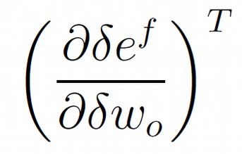
UKV - extra observations not assimilated
                               in global model
4D-Var:
•GeoCloud cloud fraction profiles (hourly, 12km thinning, assumes cloudy box if mixed cloud
and clear sky).
•Cloud fraction profiles from SYNOPs (hourly).
•Visibility from SYNOPs and METARs (hourly).
•T2m & RH2m from ~600 roadside sensors (hourly).
•Doppler radial winds from ~12 UK radars (10min).
•AMVs from NWC SAF (hourly) .
•Plans to add radar reflectivity in 2019. Radar refractivity later on.

After 4D-Var:
•radar-derived surface rain rate (15min, 5km resolution), via LHN.

                                              5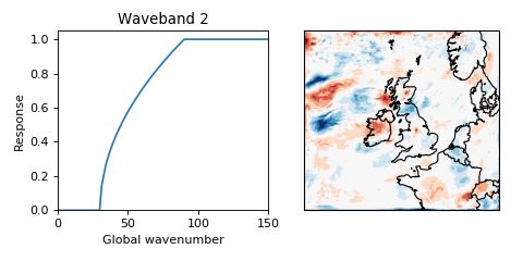
OBSERVATION
                         Previous system, 3hourly 3D-Var:
•11UTC window
                         •3 hourly cycle. Assimilation window from
OBS lost if not          T-1h30’ to T+1h30’
received by 11:45        •3D-Var. IAU applied increments over 1
•12UTC window            hour.
upper OBS
available if
                         •Lots of information per cycle.
received by 12:45
                         Hourly 4D-Var:
                         •1 Hourly cycle, less information per
                         cycle. 45’ cut-off time
                         •Better analysis fit to the observation.
                         •Loss of some observations, e.g. lower
                         part of UK sounding for 11 and 23
                         cycles.

                     6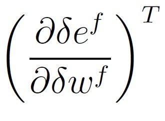
Forecast Sensitivity Observation Impact (FSOI)
•   Adjoint derived (single outer loop) observation impact.
•   Use data assimilation system to assess the impact of all OBS simultaneously. Impact of each
    OBS to forecast.
•   Don’t require a data-denial experiment (OSE) for each separate observation type.
                                                      Observation impact
        Observation innovations                      (use OBS innovation)

            (data assimilation)                        OBS sensitivities
                                                   (Adjoint data assimilation)
            Analysis increment
                                                     Analysis sensitivities
              (forecast model)                      (Adjoint forecast model)
                                             Forecast error sensitivities(Sensitivity
         Forecast in OBS space
                                                  based on quadratic norm)
Difference in the quadratic forecast error        (Adjoint PF states to OBS)
      measure (using OBS as truth)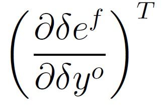
Some results
Previous 3hourly 3D-Var:
•Assessing 3 hour forecast (PS36 set-up) using observation error metric based
on synop observations of temperature, relative humidity,10-m wind speed and
log visibility.
•Negative = beneficial

In this setup:
•Openroad temperature and synop relative humidity provide largest beneficial
impact
•Buoy pressure and IASI showing largest detrimental impact.
•This project, with new results, is described in a poster from Helen Buttery
(helen.buttery@metoffice.gov.uk).

                                       8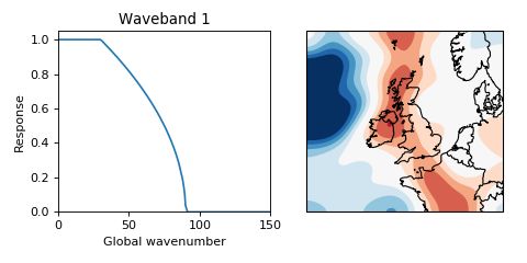
Background error covariance matrix: Tests
                                  using NMC method
• Forecast differences at same validity time (T+m)-(T+n)=Tmn
• Control run uses forecast differences from 3 hourly UKV-3DVar T63
• First tests using T21 and T63 based on hourly UKV-4DVar data and T63+Jb scaling
  (variances as T21), gave discouraging results. Lesson learnt:
   • Error structure depends on the different forecast lead times used

• Start different tests using a larger sample (4 months):
   •   T43, 1 hour time lag avoiding spin up problems
   •   T63
   •   T31, compromise between long and short time lag
   •   T31, using data where the forecast starts at 00, 06, 12, 18. To have more information from
       OBS and large differences between forecasts

                                                  9
Background error covariance matrix:
Tests using NMC method
• Tests using T63 gave neutral/slightly positive results.
• Better surface skills.
• The improvements are not sufficiently positive for operational implementation.
• All other approaches deteriorate the forecast skill.
• We assume that the error coming from the boundary can be neglected.
• Very strong approximation.
• A new approach considering error correlation between local and synoptic scales
could be beneficial.
10Development of hybrid-4DVar
11Development of hybrid-4DVar
• Treatment of large and
smaller scales in perturbations
likely to be important.
• Can remove large scales
entirely, or separate
perturbations into wavebands
and localise them separately
with different localisation
scales.
• Target for trialled hybrid-
4DVar system: March 2019.
12New cycling
Re-capturing lost sonde observations is a priority in UKV-4DVar.
•Main method:
• Extend the cut-off on 2 key cycles (11UTC & 23UTC) from 45 minutes to 80
minutes (operational since Friday 23rd February 2018).
•Alternative (under development) method:
• Use the forecast from T-2 as background (instead from T-1) for T+0.
• The T+0 cycle has 2 hours available to provide the background state to the T+2
cycle (currently is 1 hour). thus we can enhance the cut-off time.
• T+2 forecast fields are better spun-up as the time from the initialization is longer.
Thus it could been better adjusted to the initialization shock.
• The new background will be based on older observation. The background could
be less representative of the actual state.
13Conclusions
• Achievements:
• Operational hourly 4D-Var, useful for Nowcasting.
• Larger domain at high resolution, take into account more synoptic inflow.
• New types of OBS, e.g. roadside, can have large value for the forecast.
• Nobody’s perfect:
• Hourly cycles lose the assimilation of some OBS.
• Static background error covariances generated using NMC method at high resolution are not
performing well enough.
• Future plans:
• Find a way to assimilate more conventional OBS.
• Regularly apply FSOI to know the value of the OBS.
• New background error covariance matrix using Hybrid approach.
14Thank you very much
Questions?
www.metoffice.gov.uk © Crown Copyright 2018 Met OfficeReferences
• Rawlins et all. (2007). The Met Office global four-dimensional variational data
assimilation scheme. Q.J.R. Meteorol. Soc. 133, 347–362. doi: 10.1002/qj.32
• Andrew C. Lorenc and Richard T. Marriott(2014). A Forecast sensitivity to
observations in the Met Office Global numerical weather prediction. QJR Met Soc
140, 209-224
• Parrish, D. and J. C. Derber (1992). The National Meteorological Center’s Spectral
Statistical Inter-polation analysis system. Mon. Wea. Rev. 120, 1747–1763.
16Questions
• Incremental 4D-Var
• Observation thinning
• The NMC method assumptions and limits
• Introduction to FSOI
• Idea for new cycle
• Time lagging/time shifting
17Incremental 4D-VAR
• Based on the formulation of Rawlins et al. 2007
• g, first guess; a, analysis; b, background; o observations
• S is a non-linear simplification operator with tangent linear approximation S
• 4DVAR Cost function, using the simplified increments (notation avoids
sums)
(A strategy for operational implementation of 4D-Var, using an incremental
approach. Courtier et al., 1994. doi: 10.1002/qj.49712051912)
18Incremental 4D-VAR
• In the minimization a CVT (Control Variable Transform) is used.
• The B become an Identity
• New variable using CVT (swapped order):
• Ua, is the vertically adaptive grid transform (AG; Piccolo and Cullen, 2011).
19Observation thinning
• The spatial correlation between observations is used to defined the usefulness of
the observations.
• The larger are the number of the observations the higher are the computational
costs during the assimilation.
• We reduce the number of observations used taking out the less useful ones.
20The NMC method assumptions and limits
• When the differences between the forecasts are small the NMC method
underestimates variances. The analysis will be less influenced by the
observations.
• The forecasts used to compute the differences are assumed uncorrelated.
• Leads to a climatological approximation of the covariances. The error due
to the synoptic case is not taken into account.
• Large scale atmospheric states evolve with LBC.
• For LAM to reduce the influence due to LBC, forecast differences are
based on forecast using the same LBC.
21Introduction to the FSOI
Observation based forecast error norm:
Vector of observations
Vector of predicted observations
Difference in the error between background forecast and analysis forecast:
Forecast error (verified against OBS): Forecast error sensitivity:
22Idea for new cycle
T-30’ T+60’
OBS cut off T+0
• Cycle for T+0 (e.g. 01 UTC)
• Assimilation window start at T-
T-30’ T+0 T+30’ 30’ and finish at T+30’ (e.g.
Ass. Wind. T+0 between 00:30 UTC and 01:30
T+0 model time T+30’ T+120’ UTC) .
Increments • Background state from T-2 (e.g.
T+30’ T+1 T+90’ 23 UTC).
(val. Time T-30’)
Ass. Wind. cycle
• T+0 cycle will be need as
Forecast from T-1 T+1
Background T+1 T+90’ T+180’ background from T+2 (e.g. 03
(val.time T+30’) UTC). 2 hours available.
T+90’ T+2 T+150’
• Cut off time can be enlarged as
Forecast from T+0 well.
Background T+2
(val. Time T+90’)
23Time lagging/time shifting
• Time-lagging: Add perturbations with longer lead-times (forecast time), but
correct validity times.
• Time-shifting: Add perturbations that are displaced in time. It uses different
validity time, equivalent to a smoothing in time.
24You can also read


