Nekhoroshev theory and Arnold Diffusion - C. Efthymiopoulos Dipartimento di Matematica "Tullio Levi-Civita" - Dipartimento di ...

Nekhoroshev theory and Arnold Diffusion

                  C. Efthymiopoulos
     Dipartimento di Matematica “Tullio Levi-Civita”
            Università degli Studi di Padova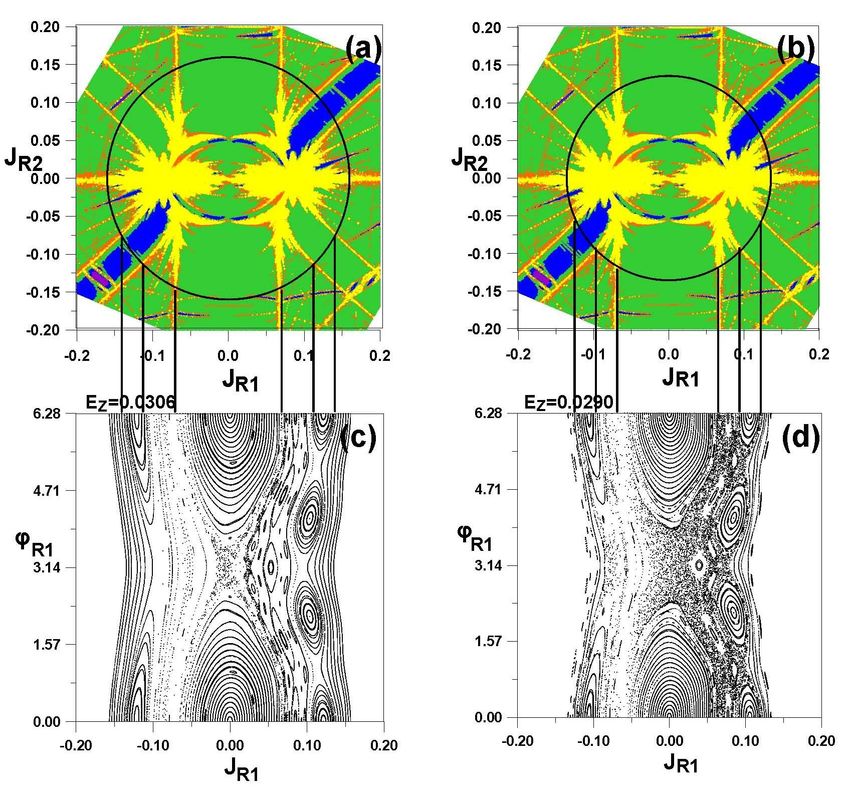

S'Agaró meeting 1995
Talk of J. Laskar and remarks by Arnold
vivid discussion (Gallavotti, Lochak, Treschev.
Simó & Delshams, de la Llave etc.)

Arnold’s example (1964)

introducing a dummy action variable J2

for μ=0, pendulum (in q,p) X 2D-tori, with frequencies

(ω1,ω2) = (J1,1)

for μ≠0, invariance of the manifold (q=p=0), which is foliated
by 2D hyperbolic tori.

Orbits started very close to a hyperbolic torus exhibit“jumps”
   in action space.

q(t)                                      p(t)
                                      t                             t

                                             p

J1(t)
                                                                        q
                                     t
                                             p

                                                                        q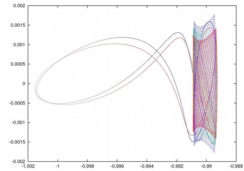

Geometric versus (semi-) analytical modelling

Geometric context:

The 2D hyperbolic tori are “whiskered”,
                           “whiskered” i.e., they possess
stable and unstable manifolds
The unstable manifold of one torus forms heteroclinic
intersections with the stable manifold of a nearby torus.
Thus a heteroclinic chain is formed.
Shadowing: near the (piecewise non-connected) parts of
the heteroclinic chain there is a real orbit shadowing the
chain
More generally: one builds an orbit shadowing a chain of
homoclinic connections on a NHIM whose existence is          (sketch by
guaranteed in a priori unstable systems (scattering map,     R. de la Llave)
see works by A. Delshams, R. de la Llave, T. Seara, M.
Gidea etc.)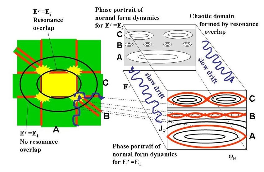

(Semi-)analytic approach (pioneered by Chirikov (1979)):

Examine the role in the evolution of the action variables of those harmonics
which contain the “pendulum” angular variable (i.e. the resonant angle, see
below). Rigorous results obtained by Chierchia and Gallavotti (1994).

  Melnikov approach

Applicability in Celestial Mechanics and Astrodynamics

Arnold diffusion: the slow diffusion of the action variables driven by
Arnold’s mechanism (motion near rhe separatrices of resonances)

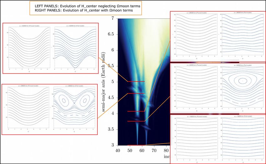
                                                             Lunisolar
                                                             resonances

                                                             (Gkolias et al.
                                                             2019)

Drift along the family of
Lyapunov orbits

(see webpage of dynamical
systems’ group, UBC, Barcelona)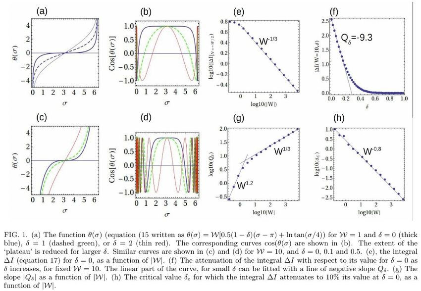

Η0(Χ,Υ)
                                                             Ηcenter(JF,uf,Jm,um)
                                                Η1(Χ,Υ,JF,uf,Jm,um) contains
(X,Y): eccentricity vector
(uf,Jf): inclination vector                     only even powers of X,Y
(um,Jm): Moon’s nodal precession

dX/dt = dY/dt = 0 by identity if X=Y=0

The subspace (JF,uf,Jm,um) remains invariant under the flow
of the full hamiltonian for all initial conditions for which X=Y=0
==> center manifold Wc

Actual satellites’ trajectories lie in the center manifold
(X~ ecosσ, Y~ esinσ)

The restriction of the flow to the center manifold is
governed by the Hamiltonian Ηcenter(JF,uf,Jm,um)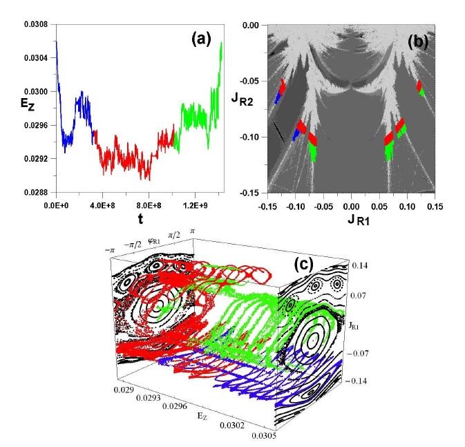

Structure of H0

    {
              Hyperbolicity

                        {     Figure-8
                              separatrix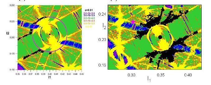

Structure of Hcenter

                                                        2π/(18.6yr)yr)

                                        {
                  precession frequencies of the satellite and of the Moon
Coefficient cos(uF)                           Coefficient cos(2uF)

                                  {
modulation of the satellite’s inclination due to the `forced’
inclination (Laplace plane)
Coefficient JF2                               Coefficient cos(2uF+ΩΩmoon)
                                  {
Separatrix of the lunisolar resonance d(2Ω-Ωmoon)/dt=0

e

                 t

    JF=O(i-i*)

                 t

Arnold’s example corresponds to a “a priori unstable” system (term
introduced in Chierchia & Gallavotti 1994).

Guzzo, Lega and Froeschlé gave the first numerical examples of Arnold
diffusion in a priori stable systems (2003, 2005)
                                                          Lega et al. 2003

Open question: prove the existence (and understand the properties) of
Arnold diffusion in a priori stable systems satisfying the necessary
conditions for the holding of Nekhoroshev theorem

       Nekhoroshev theorem

Froeschlé et al. 2000, Lega et al. 2003,2010, Guzzo et al. 2005,2009

                               I12 I 22
                 H ( I ,  )    I 3   H1
                                2 2
                              1                    
         H1                                c (k )eik 
              4  cos 1  cos 2  cos 3 |k ||k ||k | 0
                                            1   2   3

                  I2

                                 I1

Construction of the Nekhoroshev normal form

         Hamiltonian system of three degrees of freedom

Choose a point I*. Exploit analyticity in a complexified domain
                 with

Construction of the Nekhoroshev normal form

           Exponential decay of the Fourier coefficients

                   Eigenvalues of the Hessian matrix

(Quasi-)convexity: The (real symmetric) Hessian matrix M* possesses either two
eigenvalues with the same sign and one equal to zero, or three non-zero eigenvalues
with the same sign.

Construction of the Nekhoroshev normal form

1) Choose

2) Expand and “book-keep” the Hamiltonian

3) Normalization (sequence of canonical transformations)

Initial Hamiltonian

Lie series transformation

Resonant module:

for a particular choice of integer vector

Optimal normalization order
Define the sequence of smallest divisors that can appear at normalization
order r

Bound for the norms of the Lie generating functions

Propagation of small divisors

where

Norm estimates for H(r): The worst accumulation of divisors appears
in the sequence

which produces repetitions of small divisors (see C.E., Giorgilli and
Contopoulos 2004, C.E. (2012))

successive normalization steps after the order r 0

Consequence:

           (diophantine condition)

Exponentially small remainder

Size of the optimal remainder   with

hence

 C.E. (2008)

Measurements of the diffusion coefficient (Lega et al. 2003)

Power-law dependence of the diffusion coefficient on the size of the
optimal remainder

Possible to explain by the heuristic theory of Chirikov
(Cincotta, C.E., Giordano & Mestre (2014))

Global diffusion in the Arnold web (Guzzo et al. 2005)

Mechanisms to overcome the “large gap problem” (A. Delshams, R. de la Llave,
T. Seara, M. Gidea, 2000, 2003, 2006yr), Cheng and Yan 2009, Kaloshin and Zhang
2015, J.P. Marco 2016yr), etc)

possible gaps
between
the primary
wiskered tori
larger than the
excursions of
their wiskers

Double resonance

Resonance conditions:

Normal form dynamics

  JF is an integral of the Hamiltonian flow of Z alone.
  The quadratic form

  is positive definite

Constant normal form energy E’→ ellipses on the plane (JR1,JR2)

JR2
                                Island chain of
                                resonance 2
Island chain of resonance 3

                                                  Island chain of resonance 1

                                                        JR1

                                                                      φR1

Normal form +Ω remainder dynamics

Froeschlé et al. 2000, Lega et al. 2003,2010, Guzzo et al. 2005,2009

                               I12 I 22
                 H ( I ,  )    I 3   H1
                                2 2
                              1                    
         H1                                c (k )eik 
              4  cos 1  cos 2  cos 3 |k ||k ||k | 0
                                            1   2   3

Optimal Normalization order ropt

Remainder terms of order s (in the book-keeping parameter λ)

Truncated sums:

Dynamics under the flow of the normal form alone (ε=0.008))

Schematic

(see Benettin and Gallavotti (1986yr)))

                                          Dynamics of
                                          the doubly-resonant
                                          normal form
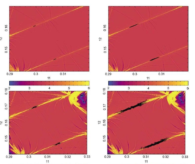
                                          + drift

A real (non-schematic) example (C.E. +Ω and Harsoula 2013)

                                                     Dynamics of
                                                     the doubly-resonant
                                                     normal form
                                                     + drift

Estimates on the speed of diffusion

We estimate how long it takes for a drift in the normal form
energy axis by an amount

Assuming normal diffusion with a per step variation ~ ||Ropt||
and step duration T

Measuring D by ensembles of chaotic orbits

“clean” variables (devoid of deformation effects,   original variables
computed by the optimal transformation)

D vs R (power-law)

Also in the single-resonant case, see Cincotta et al. 2014

Complete removal of the deformation effect
(using computer algebra ~ 10^8) terms)

Explicit knowledge of the symplectic transformation passing
from the original to “good” (i.e. deformation-free) variables

Allows to:

1. Numerically measure diffusion rates accurately and fast

2. Construct the phase portraits of the normal form dynamics

3. Visualize diffusion (and thus check for geometric
mechanisms, shadowing orbits, quantify scattering map etc)

4. Model diffusion through the normal form remainder

In summary, optimal computer-algebraic normal form calculations
provide tools and insight on how to bridge the gap between:

1. Geometric approaches (normally hyperbolic tori, whiskers
and their intersections, shadowing orbits etc.), and

2. Analytical approaches based on the modeling of the
“jumps” in action space as a scattering taking place along
homoclinic loops (e.g. Melnikov, Jeans-Landau Teller approaches,
see Chirikov, Tennyson, Wiggins, Delshams+Gelfreich+Jorba+
Seara, Benettin, Galavotti, Carati, de la Llave, Gidea etc)

(Quasi-)stationary phase approximation
M.Guzzo, C.E. and R.I.Paez (2019)

Estimate (through Melnikov integrals) the contribution of each
remainder term to the adiabatic evolution of the action variables
along homoclinic loops

Tools:

1. Choose a model in the “Nekhososhev regime”, as well as
particular initial conditions along the weakly chaotic layer
of a resonance

2. Compute the orbits (numerically)

3. Compute the optimal normal form + normalizing transformation

4. Isolate the remainder terms causing the jumps in action space

5. Visualize diffusion

Model and resonance

Non-convex but steep (depending on the choice of initial
domain in the action-space)

Orbits in the weakly chaotic layer around the 1: -1 resonance

Plane of fast drift passes through

Compute the optimal resonant normal form+remainder for various values
of ε between 0.0002, and 0.05

Transform all the orbits, find the time evolution of the “good”
(= deformation-free) variables

(Quasi-)stationary phase approximation

Normal form Hamiltonian

Remainder
                                                   Phase θ, can
                                                   be approximated
                                                   as function of the
                                                   slow angle σ only

Choose those remainder terms for which dθ/dσ ~0 in some
interval within 0

Justification: these are the only terms for which the phases do not
provide cancellations in the evolution of the action variables along
homoclinic loops

Optimal Nekhoroshev normal form

Melnikov approach

Assume the NF has the pendulum form

 Estimate the integral

Removal of the deformation

Semi-analytical vs. numerical predictions

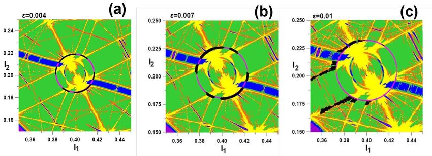
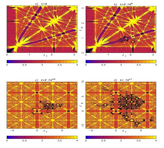
Visualization of Arnold diffusion

 A sketch
 (R. de la Llave)
                           Numerical orbit transformed in the
                           good variables

Spreading in the action space of a swarm of trajectories with
initial conditions around the hyperbolic torus of the normal form

                                        ε=0.01

Modeling of jumps
Substitute the time evolution along the NF separatrix (“a la Melnikov”)
and compute the integrals

or

for the sum (algebraic!) of all selected remainder terms

Cancellations between stationary and quasi-stationary terms

Final remarks:

Evolution in the conceptual understanding of what “Arnold diffusion”
means (driven by the applications)

Geometric versus (semi-)analytic methods (complementary)

Computer-algebra (indispensible)

Realistic estimates of the diffusion coefficient attained with methods
fully competitive to purely numerical simulations

Insight into the mechanisms which drive chaotic diffusion, as well as
the terms (in internal or external forcing) which are mostly responsible
for the observed phenomena.