Comparing Free-Throw Forms Among NBA Players Through 3D Similarity Measures

Comparing Free-Throw Forms Among NBA Players Through 3D
 Similarity Measures
 Paul Ibrahim
 Cary Academy, Cary, NC
 Paul_Ibrahim@caryacademy.org

 Abstract
In this paper, we propose a method to compare free-throw forms of various NBA players. Using
publicly available SportVU tracking data from the 2015-16 NBA season [1], we identify
instances of free-throw attempts and track the ball’s motion while it’s in the player’s hands in
order to isolate the given player’s shot form from the data. To characterize each player’s form,
we apply a multivariate kernel density estimation to the sample of the player’s free throw
attempts. Furthermore, using a k-means clustering, we attempt to categorize the multivariate
kernel density estimates across the sample of players, characterizing each cluster by the cluster
mean. We then proceed to apply a variety of three-dimensional similarity measures to the
clustered kernel density estimates, therein providing a variety of metrics by which we can assess
free-throw form similarity among NBA players.

1 Introduction
With wider adoption of the principles taught by “Moreyball” [2], the average amount of three-
point attempts per 100 possessions has dramatically risen over the course of the last decade in the
NBA [3]. Accordingly, shooting is an increasingly important skill in NBA basketball, and of
course, crucial to shooting success is player shooting form.
However, up to this point, player shooting form has predominantly existed as a qualitative study.
Most attempts at any empiricism have been primitive, confined to countable measures such as
release time, largely due to the unavailability of reliable, public data. Thus, we propose methods
through which to isolate a player’s shot form from given tracking data, and furthermore propose
viable methods through which multiple player’s three-dimensional shooting forms can be
quantitatively compared.

2 Data Processing
In our analysis, we use publicly available SportVU tracking data from the 2015-16 NBA season
[1]. Over the course of a basketball game, a player’s shooting form is evident in two distinct
situations: jump shots in the midst of gameplay, and free-throw attempts.

2.1 Confounding Variables
There are two principle, quantifiable confounding variables in the relationship between the
independent shooting form shape and a make/miss outcome: time and distance. Evaluating the
former, in jump shots over the course of a game, a player’s shooting technique is influenced by
the time left on the game clock, time left on the shot clock, and most significantly, the time they
have to release the ball before it is blocked by an opposing player. Thus, at game instances where
time is running, a player’s shooting form and their likelihood of a successful field goal attempt is
invariably influenced and altered due to the confounding variable of time. In discussion of the
latter confounder, distance, it is plausible that as distance to the basket varies, a player’s shooting
form likewise varies to some degree in order to accommodate this change.

2.2 Data Selection
Thus, in an attempt to standardize situation and eliminate probable confounding variables, we
have limited our analysis to player free-throw attempts. Because free-throws are attempted at a
fixed distance and time is removed as an influencing constraint, they serve as a medium for
functional isolation of a player’s shooting form in a purely spatial sense, thus making precise
inter-player form comparison feasible. Because of the limited nature of the dataset, we set a low
minimum of at least 10 observed free-throw attempts in the available sample of games in order
for a player to qualify as a viable subject in the study.

2.3 Data Filtering
Using the SportVU tracking data in conjunction with Basketball Reference play-by-play logs, we
can align the two datasets by game clock in order to isolate both instances of free-throw attempts
and to ascertain the identity of the attempt-taker. Filtering for the actual shooting form, we look
to capture the player’s motion which affects the velocity and angle at which the ball is released,
and get rid of all superfluous build up so as to isolate the “crux” of the shooting form for our
comparative analysis. Because SportVU player tracking attempts to track the central position of a
player at any given moment, the player’s coordinates in the course of a free-throw attempt
remain relatively sedentary. However, the ball’s center is in motion, and the trajectory of the ball
parallels the player’s shooting motion, and thus we can use the ball’s motion as a proxy for the
player’s holistic shooting form. We define the start of the shooting motion at the point where the
ball’s z-coordinate is higher than half of the player’s height1 and has continually moved up for at
least 5 frames (1/5th of a second). We define the end of the shooting motion, the release, at the
point where the ball’s x and z-coordinates have exhibited parabolic motion for at least 5 frames2.

2.4 Standardizing the Data
In order to agglomerate individual player free-throw attempt forms into a composite form and
furthermore compare composite forms between players, we first must standardize the data. We
first establish our coordinate system at a (0,0,0) origin located in the middle of the free-throw
line, where moving towards the basket would be reflected by a negative x-coordinate, motion to
the left and right parallel to the free-throw line would be reflected by negative and positive y-
coordinates, respectively, and any upward motion would be reflected by an increasingly positive
z-coordinate, dubbed in this analysis as the “radius” variable. We then can easily correct for free-
throw attempts at different baskets, establishing the near basket as the paradigm and simply
multiplying the (x,y) coordinates of attempts on the other basket by -1 in order to correct for
direction. Additionally, because we want to isolate the shot form shape independent of
handedness, we have to correct for varying dominant hands among players leading to directional
differences in shot forms. Thus, assuming a dominant right hand, we define a prototypical shot
form as temporally progressing from right to left, and thus invert the y-coordinates of all shot
forms moving left to right.

1
 Player height data from NBA.com Player Bio data [4]
2
 Because SportVU data is prone to mechanical noise, we measure signal noise in each arena's tracking device by
observing a sample of shots, after the point of release and before the ball had touched the rim, in each arena and
measured the average residual between each recorded point and the best parabolic fit. This residual average was
considered the degree of mechanical noise in each arena. If the residuals between 5 consecutive points and the best
parabolic fit are within the given arena’s residual average, it is defined as release.

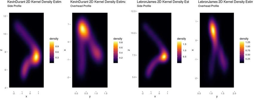
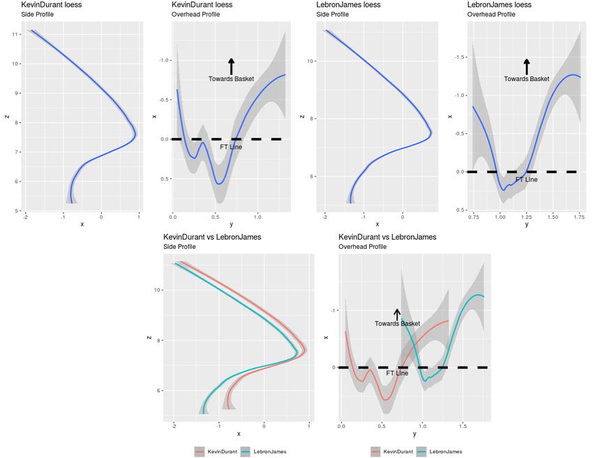
2.5 Modeling the Data
To afford the maximum possible approaches of spatial comparison, we modeled each player’s
shooting form with two methods: trivariate local regression (LOESS) and three-dimensional
kernel density estimation (KDE)3. An example is shown below in Figure 14 5.

 Figure 1: LOESS and KDE Comparative Representations

3
 In order to enable comparison across players, we had to standardize a domain across which to calculate the three-
dimensional kernel density estimate. We found that an x domain of (-2,1.75), a y domain of (-2,2), and a radius
domain of (4,10.25) encapsulated >99% of all observed points across different player shot forms. We returned
matrices of dimensions 300x320x500 from our kernel density estimates.
4
 Density values reflected in Figure 1 are not the actual probability density values, but rather were significantly
scaled up for ease of interpretability.
5
 Plots are shown in two-dimensions with two-dimensional models for the sake of clear visualization.

3 Three-Dimensional Methods of Comparison
There are a number of popularized methods for comparing trajectories in three-dimensions.
However, for our purposes, we need non-discretized methods of measuring three-dimensional
similarity. Thus, in this paper, we will focus on three principal methods to assess dissimilarity:
Frechet Distance, Euclidean Distance Matrices, and Kullback-Leibler Divergence.

3.1 LOESS Curve Frechet Distance
Because SportVU data is collected at constant time intervals, and because given players’ shot
forms vary in speed, between two players there doesn’t exist an absolute frame of reference if we
want to purely compare the actual shot form disregarding time. Thus, to overcome this obstacle,
we can use the LOESS model we constructed in section 2.5. Systemically sampling 500 points
from each player’s LOESS fit6, we can use the Frechet Distance algorithm to map each point to
its approximate corresponding point on the other player’s form curve and calculate a similarity
measure between the two player’s curves [5]. The most significant drawback of this method is
that because it can only be accomplished by modeling each player’s shot form as a consolidated
LOESS curve, the similarity measure functionally compares the mean of each player’s shot form
rather than accounting for potential variance and inconsistencies across the sample of each
player’s shot forms.

3.2 Bin Difference
Loosely paralleling the methodology outlined in section 3.1, to estimate the difference between
two player’s shot forms, we can simply calculate the bin difference between two three-
dimensional arrays [6]. Using the 3D KDE model established in section 2.5, we can find the
absolute difference in density estimate per corresponding cell between the two players’ KDE
arrays, and sum these absolute differences together to represent a holistic similarity measure.

3.3 Kullback-Leibler Divergence
The final, most robust method we use to estimate shot form similarity is calculating the three-
dimensional Kullback-Leibler Divergence (KLD) between two player’s shot forms. Kullback-
Leibler Divergence is a method through which one can assess the similarity between two
probability distributions [7]. The formula to calculate a three-dimensional Kullback-Leibler
Divergence is given below in Formula 1:
 ∞
 ( )
 ( , ) = ∭ ( ) log ( ) 
 −∞ ( )
 Where = ( , , ), = ( , , ), ( ) represents the target probability distribution and ( ) represents the
 competing probability distribution

Our 3D KDE model constructed in section 2.5 is a three-dimensional probability density function
that integrates to 1; thus, we can substitute our determined three-dimensional kernel density
estimates for two given players in lieu of probability distributions ( ) and ( ) while
maintaining the integrity of the Kullback-Leibler Divergence.

 Table 1: Comparative Table of Kevin Durant and Lebron James7

Using our collected sample of players, we can deduce the correlogram below, showing the
distribution and correlation between our various similarity measures and free-throw percentage.

 Figure 2: Similarity Measures Correlogram8

7
 Player 1 Treated as Target Distribution
8
 In Bin Difference and LOESS Distance calculations, composite average of all player shooting forms was treated as
the base form for comparison. In Kullback-Leibler Divergence calculations, composite average of all player
shooting forms is treated as the target probability distribution.

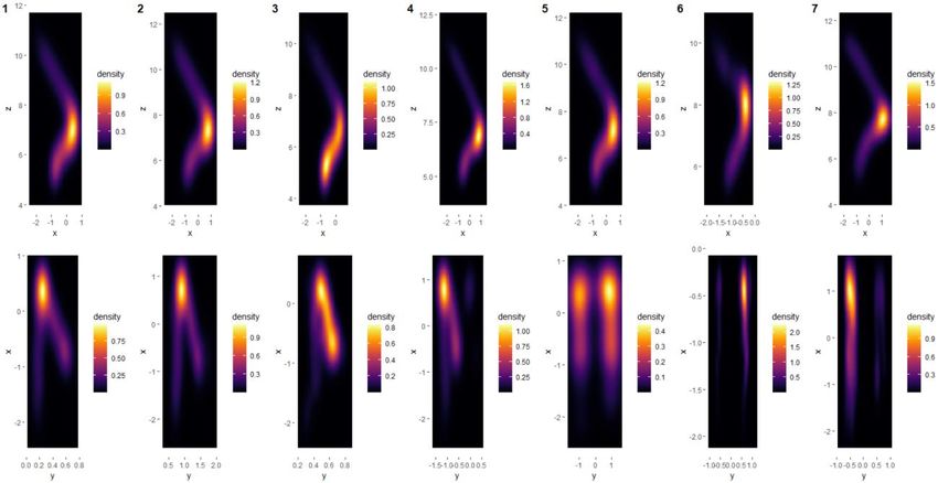
4 Clustering Shot Forms
In order to conduct a more generalized analysis on player shot forms, we can sort them into
clusters using the k-means clustering algorithm. Using the elbow method, we identify that the
sum of squares is minimized for our sample of players at 7 clusters. Thus, arranging our sample
of player shot forms into 7 clusters, we can further characterize each cluster by the cluster mean,
resulting in the following shot forms:

 Figure 3: Clustered Shot Forms from Side and Overhead Vantage

Repeating the methodology outlined in section 3, we compare each cluster to the composite
average of all player shooting forms with each of the outlined similarity measures9.
 Table 2: Cluster Comparative Table7

5 Conclusion
Throughout this paper, we have proposed methods to compare free-throw forms of various NBA
players, both individually and generalized within clusters. We have outlined viable methods of
producing three-dimensional similarity measures, calculating inter-player/cluster three-
dimensional Frechet Distance, three-dimensional Bin Difference, and three-dimensional
Kullback-Leibler Divergences.

References

[1] linouk23. “linouk23/NBA-Player-Movements.” GitHub, 19 Sept. 2016,
 github.com/linouk23/NBA-Player-
 Movements/tree/master/data/2016.NBA.Raw.SportVU.Game.Logs

[2] Dubin, Jared. “Nearly Every Team Is Playing Like The Rockets. And That's Hurting The
 Rockets.” FiveThirtyEight, FiveThirtyEight, 20 Dec. 2018,
 fivethirtyeight.com/features/nearly-every-team-is-playing-like-the-rockets-and-thats-
 hurting-the-rockets/.

[3] “NBA League Averages - Per 100 Possessions.” Basketball, 2020, www.basketball-
 reference.com/leagues/NBA_stats_per_poss.html.

[4] “Players Bios.” NBA Stats, 2020, stats.nba.com/players/bio/.

[5] Bereg, Sergey, et al. “Simplifying 3D Polygonal Chains Under the Discrete Fréchet
 Distance.” Lecture Notes in Computer Science LATIN 2008: Theoretical Informatics, pp.
 630–641., doi:10.1007/978-3-540-78773-0_54.

[6] Krakov, David, and Dror G. Feitelson. “Comparing Performance Heatmaps.” Job Scheduling
 Strategies for Parallel Processing Lecture Notes in Computer Science, 2014, pp. 42–61.,
 doi:10.1007/978-3-662-43779-7_3.

[7] squared2020. “An Example in Kullback-Leibler Divergence.” Squared Statistics:
 Understanding Basketball Analytics, 7 Feb. 2019, squared2020.com/2019/02/07/an-
 example-in-kullback-leibler-divergence/.