NOTALLGOALSARECREATEDEQUAL - DIVA
←
→
Page content transcription
If your browser does not render page correctly, please read the page content below
Linköping University | Department of Computer and Information Science
                                 Master’s thesis, 30 ECTS | Datateknik
                               2021 | LIU-IDA/LITH-EX-A--21/008--SE

  Not All Goals Are Created Equal
  –Evaluating Hockey Players in the NHL Using Q-Learning with a
  Contextual Reward Function

  Värdering av hockeyspelare i NHL med hjälp av Q-learning med
  en kontextuell belöningsfunktion

  Jon Vik

  Supervisor : Niklas Carlsson
  Examiner : Patrick Lambrix

                                                      Linköpings universitet
                                                        SE–581 83 Linköping
                                               +46 13 28 10 00 , www.liu.se
Upphovsrätt
Detta dokument hålls tillgängligt på Internet - eller dess framtida ersättare - under 25 år från publicer-
ingsdatum under förutsättning att inga extraordinära omständigheter uppstår.
Tillgång till dokumentet innebär tillstånd för var och en att läsa, ladda ner, skriva ut enstaka ko-
pior för enskilt bruk och att använda det oförändrat för ickekommersiell forskning och för undervis-
ning. Överföring av upphovsrätten vid en senare tidpunkt kan inte upphäva detta tillstånd. All annan
användning av dokumentet kräver upphovsmannens medgivande. För att garantera äktheten, säker-
heten och tillgängligheten finns lösningar av teknisk och administrativ art.
Upphovsmannens ideella rätt innefattar rätt att bli nämnd som upphovsman i den omfattning som
god sed kräver vid användning av dokumentet på ovan beskrivna sätt samt skydd mot att dokumentet
ändras eller presenteras i sådan form eller i sådant sammanhang som är kränkande för upphovsman-
nens litterära eller konstnärliga anseende eller egenart.
För ytterligare information om Linköping University Electronic Press se förlagets hemsida
http://www.ep.liu.se/.
Copyright
The publishers will keep this document online on the Internet - or its possible replacement - for a
period of 25 years starting from the date of publication barring exceptional circumstances.
The online availability of the document implies permanent permission for anyone to read, to down-
load, or to print out single copies for his/hers own use and to use it unchanged for non-commercial
research and educational purpose. Subsequent transfers of copyright cannot revoke this permission.
All other uses of the document are conditional upon the consent of the copyright owner. The publisher
has taken technical and administrative measures to assure authenticity, security and accessibility.
According to intellectual property law the author has the right to be mentioned when his/her work
is accessed as described above and to be protected against infringement.
For additional information about the Linköping University Electronic Press and its procedures
for publication and for assurance of document integrity, please refer to its www home page:
http://www.ep.liu.se/.
© Jon VikAbstract
Not all goals in the game of ice hockey are created equal: some goals increase the
chances of winning more than others. This thesis investigates the result of constructing
and using a reward function that takes this fact into consideration, instead of the common
binary reward function. The two reward functions are used in a Markov Game model with
value iteration. The data used to evaluate the hockey players is play-by-play data from the
2013-2014 season of the National Hockey League (NHL). Furthermore, overtime events,
goalkeepers, and playoff games are excluded from the dataset. This study finds that the
constructed reward, in general, is less correlated than the binary reward to the metrics:
points, time on ice and star points. However, an increased correlation was found between
the evaluated impact, and time on ice for center players. Much of the discussion is devoted
to the difficulty of validating the results from a player evaluation due to the lack of ground
truth. One conclusion from this discussion is that future efforts must be made to establish
consensus regarding how the success of a hockey player should be defined.Acknowledgments
I want to thank my supervisor, Niklas Carlsson, and my examiner, Patrick Lambrix, for their
unending enthusiasm for this work. I also want to express my gratitude to Nahid Shahmehri
for her warm welcoming to ADIT. Thank you to Linn Mattson for being the opponent for this
thesis after all this time.
This thesis would not have been possible without the help from many people in my life. My
endless gratitude goes to Ulla Högstadius and Rickard Wedin. Thank you to Sofia Edsham-
mar. Thank you to my mother Lena, my father Gunnar, my brother Olov, and my partner
Rebecca. I will be forever grateful to all of you.
ivContents
Abstract iii
Acknowledgments iv
Contents v
List of Figures vii
List of Tables viii
1 Introduction 1
1.1 Motivation . . . . . . . . . . . . . . . . . . . . . . . . . . . . . . . . . . . . . . . . 1
1.2 Aim . . . . . . . . . . . . . . . . . . . . . . . . . . . . . . . . . . . . . . . . . . . . 2
1.3 Research Questions . . . . . . . . . . . . . . . . . . . . . . . . . . . . . . . . . . . 2
1.4 Delimitations . . . . . . . . . . . . . . . . . . . . . . . . . . . . . . . . . . . . . . 2
1.5 Research Method . . . . . . . . . . . . . . . . . . . . . . . . . . . . . . . . . . . . 2
1.6 Outline . . . . . . . . . . . . . . . . . . . . . . . . . . . . . . . . . . . . . . . . . . 3
2 Background 4
2.1 Hockey Rules . . . . . . . . . . . . . . . . . . . . . . . . . . . . . . . . . . . . . . 4
2.2 Hockey Concepts . . . . . . . . . . . . . . . . . . . . . . . . . . . . . . . . . . . . 7
3 Theory 11
3.1 Markov Game Model . . . . . . . . . . . . . . . . . . . . . . . . . . . . . . . . . . 11
3.2 Alternating Decision Tree . . . . . . . . . . . . . . . . . . . . . . . . . . . . . . . 12
3.3 Value Iteration . . . . . . . . . . . . . . . . . . . . . . . . . . . . . . . . . . . . . . 12
4 Related Work 14
4.1 Related Approaches and Problems . . . . . . . . . . . . . . . . . . . . . . . . . . 14
5 Method 17
5.1 The Work of Routley and Schulte . . . . . . . . . . . . . . . . . . . . . . . . . . . 17
5.2 Data Pre-Processing . . . . . . . . . . . . . . . . . . . . . . . . . . . . . . . . . . . 21
5.3 Reward Function . . . . . . . . . . . . . . . . . . . . . . . . . . . . . . . . . . . . 22
5.4 Merging Existing Code Base with the Reward Function . . . . . . . . . . . . . . 24
5.5 Three Stars Metric . . . . . . . . . . . . . . . . . . . . . . . . . . . . . . . . . . . . 24
6 Results 26
7 Discussion 33
7.1 Results . . . . . . . . . . . . . . . . . . . . . . . . . . . . . . . . . . . . . . . . . . 33
7.2 Method . . . . . . . . . . . . . . . . . . . . . . . . . . . . . . . . . . . . . . . . . . 34
7.3 The Work in a Wider Context . . . . . . . . . . . . . . . . . . . . . . . . . . . . . 35
v8 Conclusion 36
Bibliography 37
9 Appendix 40
9.1 Weighted Metrics Correlations . . . . . . . . . . . . . . . . . . . . . . . . . . . . 40
9.2 Top 30 Weighted Points . . . . . . . . . . . . . . . . . . . . . . . . . . . . . . . . . 42
9.3 Weighted Points versus Traditional Points . . . . . . . . . . . . . . . . . . . . . . 42
9.4 Top 25 Players . . . . . . . . . . . . . . . . . . . . . . . . . . . . . . . . . . . . . . 43
viList of Figures
1.1 Goal frequency for each minute of the first three periods in the NHL during the
2013-2014 season. . . . . . . . . . . . . . . . . . . . . . . . . . . . . . . . . . . . . . . 1
1.2 CCDF of the time between all goals scored in period one, two and three during
the 2013-2014 NHL season. . . . . . . . . . . . . . . . . . . . . . . . . . . . . . . . . . 1
2.1 Hockey rink with the three different zones. The zone perspective is from the team
with the goaltender in the left goal. . . . . . . . . . . . . . . . . . . . . . . . . . . . . 6
5.1 Subset of events in a tree. . . . . . . . . . . . . . . . . . . . . . . . . . . . . . . . . . . 19
5.2 Reward distribution over time and goal difference. Each bin is two minutes long.
Less than three observations for each bin are left out. . . . . . . . . . . . . . . . . . 23
5.3 Negative reward distribution over time and goal difference. Each bin is two min-
utes long. Less than three observations for each bin are left out. . . . . . . . . . . . 23
5.4 Reward distribution over time and manpower difference. Each bin is two minutes
long. Less than three observations for each bin are left out. . . . . . . . . . . . . . . 24
5.5 Cumulative distribution function of the reward. . . . . . . . . . . . . . . . . . . . . 24
5.6 Venn diagram over the relevant classes concerning the three stars metric. . . . . . . 25
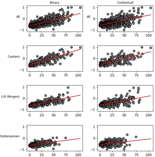
6.1 Impact vs. points for different skater positions and different reward functions. . . 27
6.2 Impact vs. time on ice in hours. . . . . . . . . . . . . . . . . . . . . . . . . . . . . . . 28
6.3 Impact vs. star points. Players that have never been on the three stars list are
excluded. . . . . . . . . . . . . . . . . . . . . . . . . . . . . . . . . . . . . . . . . . . . 29
9.1 Weighted points versus traditional points. . . . . . . . . . . . . . . . . . . . . . . . . 42
viiList of Tables
2.1 NHL teams during the 2013-2014 season. . . . . . . . . . . . . . . . . . . . . . . . . 5
2.2 Top 30 players by star points. . . . . . . . . . . . . . . . . . . . . . . . . . . . . . . . 9
2.3 Conventional metrics and their abbreviations. . . . . . . . . . . . . . . . . . . . . . 10
2.4 Selection of NHL awards. . . . . . . . . . . . . . . . . . . . . . . . . . . . . . . . . . 10
5.1 Action events committed by players in the play-by-play table. . . . . . . . . . . . . 18
5.2 Start and end events in the play-by-play table. . . . . . . . . . . . . . . . . . . . . . 18
5.3 The implemented definition of the missing metricTable. . . . . . . . . . . . . . . 22
6.1 Three stars precision and recall. . . . . . . . . . . . . . . . . . . . . . . . . . . . . . . 29
6.2 Maximal information-based correlation (MIC) between the two impacts, star
points and traditional metrics. Recall from Section 2.2 that GP are games played,
P are points, +/- is the plus-minus metric, and TOI is time on ice. . . . . . . . . . . 30
6.3 Selection of recipients and runner-ups of seasonal trophy awards with impacts
and traditional metrics. The rewards are noted with the following symbols: Most
points *, best first-year player †, best defensive forward ‡, most valuable player of
the regular season §, best defenseman ||, most goals ¶. . . . . . . . . . . . . . . . . 31
9.1 Maximal information-based correlation (MIC) between the two impacts, star
points, weighted plus minus, weighted points and traditional metrics. . . . . . . . 40
9.2 Weighted points and ranking difference to traditional points. . . . . . . . . . . . . . 41
9.3 Top 25 players using contextual reward. . . . . . . . . . . . . . . . . . . . . . . . . . 43
viii1 Introduction
The introduction section gives an account for why this work is useful. Next, the aim of this
thesis is specified with research questions, delimitations and research method. Last, an out-
line for the different chapters are provided.
1.1 Motivation
When evaluating the performance of ice hockey players in the National Hockey League (NHL),
it is most common to use metrics like the number of goals and assists over a season1 . One
weakness with such metrics is that they do not take into consideration the context in which
the goal was scored in. For instance, a goal scored when you are in the lead with 9–2 at the
end of the game is most likely not crucial for winning. In contrast, a goal when the score is
2–2 with fifteen seconds left of the game is of more importance for winning. In addition to
this, goals are not evenly distributed over time. This becomes apparent when looking at all
goals scored during regular time in Figure 1.1. It appears that fewer goals are scored in the
beginning of each period and more goals are scored towards the end of first and third period.
Figure 1.1: Goal frequency for each minute Figure 1.2: CCDF of the time between all
of the first three periods in the NHL during goals scored in period one, two and three
the 2013-2014 season. during the 2013-2014 NHL season.
1 https://www.eliteprospects.com/league/nhl
11.2. Aim
To further illustrate this, the complementary cumulative distribution function (CCDF) can be
seen in Figure 1.2. Here, the sudden directional change at the end of the curves for period
one and three means that the time between goals decreases notably at these two parts of the
game. This is due to the previously mentioned fact that more goals are scored towards the
end of first and third period.
This thesis aims to find the value of goals by looking at what goals increase the chance of
winning a game. This information will then also be used to evaluate players by looking at
how important their actions are with regards to winning a game.
The results of this thesis can be used by teams to acquire players that add the most value to
the team. Moreover, the data can be used by TV analysts to provide more insightful statistics
to the viewers.
1.2 Aim
The underlying purpose of the thesis project is to investigate if a contextual reward function
can be of use when trying to find hockey players in the NHL who contribute to high value
goals. Specifically, the results are compared to evaluating hockey players with a standard
binary reward function.
The results from this experiment can be of interest for hockey coaches that want to acquire,
or gain insight on, hockey players who contribute to game deciding goals. In addition to
this, game- or TV analysts may use the results to get better understanding for how different
players perform in different situations.
As an example, the team captain of the Washington Capitals, Alexander Ovechkin, stood
for the most tying- and lead taking goals during the 2013/2014 NHL season. In contrast,
Ovechkin is in place 29 on the list of most goals scored when your team is already in the lead.
In similar fashion, the number one goal scorer when the team is already in the lead is Max
Pacioretty of the Montréal Canadiens, who is not top 10 on lead taking goals, or even top
100 on the tying goals list. This hints of Ovechkin being more of a clutch player, stepping
up when needed, than Pacioretty. However, with value iteration and a contextual reward
function there are more subtleties to be found than just about the goal scorers. With this
algorithm one finds out how every player contributes to different goals, and not just the one
who make them.
1.3 Research Questions
1. How can a contextual reward function for a scored goal be constructed?
2. How does a contextual reward function affect the estimated impact of player actions?
1.4 Delimitations
This work will be limited to the Markov Game model and value iteration approach of Routley
et. al. [22]. Furthermore, because of the time consuming algorithms, the player impact esti-
mation will only be carried out on one of NHL seasons. Additionally, the 2013/2014 season
was chosen because it was the most recent complete season in the dataset [22]. Goalkeepers
are excluded from the player evaluation because of the limited data that describe the actions
of goalkeepers.
1.5 Research Method
A literature study of the work of Routley and Schulte [22] was made. In addition to that, the
underlying theory and algorithms in the previously mentioned paper were studied. Then, the
21.6. Outline
quantitative research and implementation of constructing a new contextual reward function.
This reward function was unit tested to ensure correctness. Further, this reward function
was integrated with the code from Routley and Schulte [22]. Last, the new contextual re-
ward function was compared to the original binary reward function, common metrics and
the opinions of experts. The results using the contextual reward function were verified by
their similarity to the original results of Routley and Schulte [22].
1.6 Outline
After the introduction follows a chapter with background information about hockey rules and
concepts, as well as the available data. Next, the theory chapter provides the formal theory,
as well as its previously made adaptation, needed before doing the work described in the
following method chapter. The method chapter describes the reward function construction
and the integration of it and the existing code from Routley and Schulte [22]. Furthermore,
the results are later presented in the form of plots and tables. Last, the method, results and
difficulties are presented in the discussion chapter.
32 Background
The background chapter aims to give the reader the information needed to understand the
domain of ice hockey. This involves basic rules, season structure, and other necessary con-
cepts.
2.1 Hockey Rules
The rules from this section are taken from the NHL official rules book [8]. It is worth noting that
the rules and number of teams have changed over the years. But because only the 2013/2014
season will be analyzed, the rules used in this season are presented instead of the most recent
ones. For instance, after the 2014/2015 NHL season, the overtime was played with three
skaters from each team on the ice. Nevertheless, most rules and concepts stay the same.
Season Structure
The NHL in North America divides the hockey season into two parts: the regular season and
the playoffs, also known as the Stanley Cup playoffs. During the regular season, the 30 NHL
teams play against each other and the winning team gets two points if they win, and zero
points if they lose. The exception to this is in the case of a tie after three periods. Then, the
team that loses gets one point. If there is no overtime, the losing team gets zero points. Each
team tries to acquire enough points during each of their 82 regular season games to be one
of the 16 teams that go to the playoffs. The names of all teams in the NHL are available in
Table 2.1.
Game Structure
Each game consists of three 20 minute periods in regulation time and starts with six players from
each team on the ice, five skaters and one goalkeeper. The team with the most goals at the end
of regular time is deemed the winner. In case of a tie, the game goes into overtime, where
there are only four skaters and one goalkeeper from each team, to begin with. In addition
to this, the overtime period is played as sudden death, also known as golden goal, meaning
that if any of the teams scores, the game is ended and the scoring team is the winner of the
game. If there is no goal during the five minutes of overtime, the game goes to a shootout. In
42.1. Hockey Rules
Short Name Name
TOR Toronto Maple Leafs
MTL Montreal Canadiens
WSH Washington Capitals
CHI Chicago Blackhawks
WPG Winnipeg Jets
EDM Edmonton Oilers
PHI Philadelphia Flyers
BUF Buffalo Sabres
DET Detroit Red Wings
ANA Anaheim Ducks
COL Colorado Avalanche
TBL Tampa Bay Lightning
BOS Boston Bruins
NJD New Jersey Devils
PIT Pittsburgh Penguins
CGY Calgary Flames
NSH Nashville Predators
STL St. Louis Blues
LAK Los Angeles Kings
MIN Minnesota Wild
FLA Florida Panthers
DAL Dallas Stars
NYR New York Rangers
PHX Phoenix Coyotes
VAN Vancouver Canucks
SJS San Jose Sharks
OTT Ottawa Senators
NYI New York Islanders
CAR Carolina Hurricanes
CBJ Columbus Blue Jackets
Table 2.1: NHL teams during the 2013-2014 season.
a shootout, each team selects three skaters that try to score on the goalkeeper of the opposing
team with no other players on the ice. In case of a tie after a total of six shootouts, both teams
choose one skater each for a sudden death round. If both skaters score or fail to score, the
process is repeated until there is a winning team.
Compared to the fixed schedule of the regular season, the playoffs are played as an elim-
ination tournament of four rounds. In every round, two teams play against each other in
a best of seven games series. As a consequence, the team that is first to win four of those
seven games will advance to the next round. Thus, the losing team is eliminated from the
playoffs. The tournament is played until there is only one team left that then are the winners
of the Stanley Cup of that season. Unlike the regular season games, playoff game overtimes
are always played with five skaters on the ice without shootouts. Instead, overtime is played
as repeated regular 20 minute periods, but with the difference that the periods are played in
sudden death.
Playing Positions
The hockey player positions are often divided into forwards, defensemen and goalkeeper. The
goalkeeper is also known as the goaltender or goalie. The forwards consist of a left winger,
center and a right winger. The forwards are usually the players that score the majority of the
52.1. Hockey Rules
goals. Similarly, the defensemen consist of a left defenseman and a right defenseman and,
as the name suggests, bear most of the defensive responsibility together with the goalkeeper.
The goalkeeper does not count as a skater on the ice. Instead, the goalkeeper has special
equipment such as a different helmet, large protective gear, and special skates for stability.
The most important task of the goalkeeper is to block the incoming shots on goal from the
opposing team.
In spite of players having different positions, there is nothing stopping a forward from
taking a more defensive responsibility or a defenseman from scoring.
Penalty
A potential rule violation may lead to a penalty on the player who committed the rule vio-
lation. As a consequence, the player that made the infraction can be penalized with either
a minor penalty of two minutes, a double minor of a total of four minutes, a major penalty of
five minutes, a major penalty of 10 minutes, or a game misconduct. For all cases but the game
misconduct, the player is sent to the penalty box for the time of the penalty, leaving the team
one player short on the ice. Minor penalties are ended early in case the team on the power
play scores a goal. In the case of a game misconduct, the player is ejected from the game and
one of his teammates has to sit in the penalty box instead. There can be multiple players from
the same team in the penalty box at the same time.
If a penalty is called against a team that is not in possession of the puck, it is called a delayed
penalty. As a result, the game will not be stopped until the opposing team gains possession of
the puck or there is a stoppage of the game due to something else. For instance, a stoppage
occurs when the puck leaves the playing area, the goaltender holds on to the puck after a
saved shot, etc.
Figure 2.1: Hockey rink with the three different zones. The zone perspective is from the team
with the goaltender in the left goal.
62.2. Hockey Concepts
2.2 Hockey Concepts
Manpower
From the start of a hockey game, there are always five skaters and one goaltender on the ice.
The number of players allowed on the ice during a moment in the game changes as a result
of penalties. The number of skaters on the ice is referred to as the manpower. Furthermore,
manpower is often denoted as 5-on-5 when both teams have five skaters on the ice, making
the manpower even. Naturally, when one team is down one player due to a penalty, it is
denoted 5-on-4, etc. It is called boxplay when a team has fewer players on the ice than the
other team. If a team scores in boxplay, it is called a shorthanded goal. On the contrary, the
team with one player more than the opposing team is then on powerplay. A goal scored on
powerplay is called a powerplay goal.
Puck Possession
A skater on the ice has possession of the puck if the skater is the last one who touched the
puck. Puck possession is not to be confused with puck control, where the skater must move
the puck with stick, hand, or feet.
Pulling the Goalie
It is not only during penalties that one might observe an extra skater on the ice. It is not
uncommon that a team substitutes its goalkeeper for an extra attacker at some point during
the game. This is known as pulling the goalie. The substitution of a goalkeeper for an extra
skater can be done at any time. This often happens during a delayed penalty where there is a
low risk of the puck finding its way to the goal without the opposing team having possession
of it. Consequently, many teams substitute their goalkeeper for an extra attacker to gain an
advantage over the other team. It is also common that this substitution is done by a team that
is trailing a few goals. This is done in a last attempt to tie the game, thus taking it to overtime
and creating a chance to win the game.
Sequence
A sequence is defined as all the events that happen between the event where one team gains
possession of the puck, to the event that the same team loses the possession. This definition
facilitates when talking about all the events where one of the teams is attacking.
Zones
The playing field can be divided into three different zones: The defensive, neutral and offensive
zone. As can be seen in Figure 2.1, the neutral zone is in the middle of the hockey rink and is
the same for both teams. In contrast, the defensive and offensive zone depends on the team
in question. In Figure 2.1, the zones are from the perspective of the team with its goaltender
in the left goal. If one were to see it from the perspective of the opposing team with the
goaltender in the right goal, the defensive and offensive zone would be switched. Intuitively,
the defensive zone has the goal a team wants to defend, whereas the offensive zone has the
goal a team wants to score on.
The NHL Entry Draft
The NHL Entry Draft was introduced to the league in 1963. The draft became a fair way to
draft young players between the age of 18 and 21 to the NHL. Essentially, the draft is a lottery
system that decides the selection order of new players. Furthermore, the teams that had the
72.2. Hockey Concepts
worst results of the season get increased chances of an early draft pick and vice versa. This
way, poor performing teams have an improved opportunity to draft the most talented young
players that could potentially boost the performance of the team. Draft selection order can
also be traded between teams as a way to acquire senior players 1 .
Three Stars
Three stars of the game is a way of giving recognition to the three best players of a game. The
three best players are chosen by an external party. For example, home broadcasters, local
sports journalists, and sponsors can be found as third parties in the NHL game summary
sheets 2 . The list is ordered descendingly with the first star being the best player [29]. Each
player is given points depending on their placement in the list. 30 points are given to the first
star, 20 points to the second star, and 10 points to the third star. This way, one can compare
the performance of players between seasons as reflected by the three stars list. The top NHL
players in regards to star points can be found in Table 2.2.
The three stars list is entirely subjective. Therefore, the best players are not always
awarded a star. For instance, retiring players have been put on the three stars list as ap-
preciation for their long career, rather than their performance during the game. Even the
crowd has appeared on the three stars list for their enthusiasm during the game [29].
1 https://web.archive.org/web/20010128131400/http://nhl.com/futures/drafthistory.
html
2 http://www.nhl.com/scores/htmlreports/20122013/GS020483.HTM – Example game summary.
82.2. Hockey Concepts
Player Pos Star Points
Sidney Crosby C 670
Ryan Getzlaf C 570
Alex Ovechkin R 550
Corey Perry R 510
Anze Kopitar C 490
Matt Duchene C 480
Joe Pavelski C 450
Jamie Benn L 450
Alexander Steen L 440
Shea Weber D 420
Ryan Johansen C 420
Patrick Sharp L 400
Joe Thornton C 400
Jonathan Toews C 380
Jason Pominville R 370
Tyler Seguin C 370
Jason Spezza C 370
Claude Giroux C 370
Martin St. Louis R 350
Ryan Kesler C 350
Jeff Skinner L 350
Blake Wheeler R 350
Evgeni Malkin C 350
David Krejci C 350
Zach Parise L 340
Andrew Ladd L 340
John Tavares C 320
Phil Kessel R 320
Brandon Dubinsky C 320
Mats Zuccarello L 320
Table 2.2: Top 30 players by star points.
Common Metrics
Common metrics used in the NHL are basic statistics that in some way describe the actions of
players. From now on, the common metric may also be referred to as traditional metrics in
order to distinguish them from more advanced and lesser used metrics. The most common
metrics and their abbreviations can be found in Table 2.3. These specific metrics are usually
used when looking at players over entire seasons or careers. The traditional metrics provide
a quick and simple way of knowing how successful a player has been.
Many of the metrics are self-explanatory when looking at the names. But some need an
explanation for the one unfamiliar with sports. Here, points are given to players who either
score a goal or make an assist. Assist is the word for passing the puck to a teammate who then
shortly scores a goal. One point is given for an assist and one point for a goal. These points
are then aggregated in the points metric. The game winning goal is defined as the last goal
of the game that made the game go from a tie to a lead from the perspective of the winning
team. The plus-minus, or ’+/-’, metric denotes the relationship between scored and conceded
goals while the player is on the ice. One point is added to the metric if a goal is scored and
the player is on the ice. Similarly, one point is deducted if the player is on the ice while a goal
is conceded.
92.2. Hockey Concepts
Abbreviation Metric
GP Games Played
G Goals
A Assists
P Points
+/- Plus-minus
TOI Time On Ice
PIM Penalty Minutes
PPG Power Play Goals
SHG Short-Handed Goals
GWG Game Winning Goals
Table 2.3: Conventional metrics and their abbreviations.
Awards
At the end of each NHL season, players who have excelled at their work are eligible for
receiving an award. These rewards come in the form of trophies. Some of the trophy winners
a selected based on statistics, such as the Art Ross Trophy, which is awarded to the player with
the most points. With other trophies, such as the Hart Memorial Trophy, the recipient is chosen
based on the voting of North American journalists that are members of the Professional Hockey
Writers’ Association 3 . In Table 2.4 is a selection of the trophies awarded after each season.
These rewards will be compared to the results in Chapter 6.
Award Description Recipient Runner-ups
Art Ross Trophy Most points Sidney Crosby Ryan Getzlaf
Calder Memorial Trophy Best first-year player Nathan MacKinnon Tyler Johnson, Ondrej Palat
Frank J. Selke Trophy Best defensive forward Patrice Bergeron Anze Kopitar, Jonathan Toews
Hart Memorial Trophy Most valuable player of regular season Sidney Crosby Ryan Getzlaf, Claude Giroux
James Norris Memorial Trophy Best defenceman Duncan Keith Zdeno Chara, Shea Weber
Maurice "Rocket" Richard Trophy Most goals Alexander Ovechkin Corey Perry
Table 2.4: Selection of NHL awards.
3 https://www.thephwa.com/
103 Theory
The mathematical models that form the underlying foundation for the algorithms used are
presented in this chapter.
3.1 Markov Game Model
In 1994 Littman [10] proposed the use of Markov Games instead of Markov Decision Processes [6]
in reinforcement learning. As a result of using Markov Games, it became possible to formally
describe a mathematical model that has two adaptive agents that have opposed goals. An
adaptive agent responds to the environment and different agents. Furthermore, two opposed
goals can be two hockey teams that strive towards having a higher score than the other team
at the end of the game.
Littman [10] describes the essential characteristics of a Markov Game as the set of states
S, multiple action sets A1 , . . . , An , where each agent has its own action set. The transition
function,
T : S ˆ A Ñ PD (S) (3.1)
describes how taking action A in state S leads to a new state decided by PD (S), which is the
set of discrete probability distributions over S. The necessity for PD (S) comes from the fact
that taking an action in some state may not always lead to the same new state. For instance,
an ice hockey shot may lead to a goal or a goaltender save, which are in two different states.
The last requirement of a Markov Game is the reward function of each agent. The reward
function describes desirable agent behavior and will guide it towards taking the best actions.
For example, scoring a goal is good and will result in a high reward, whereas conceding a
goal is bad and will not yield any reward, sometimes even a negative reward, i.e. penalty, is
given in such cases. The reward function is formally described as:
R i : S ˆ A1 ˆ . . . ˆ A k Ñ < (3.2)
The Ri subscript emphasizes that each agent has its own reward function that may be dif-
ferent from the reward functions of other agents. The reward function is then used to guide
the agents to desirable behavior. This can be done for instance by instructing the agents to
113.2. Alternating Decision Tree
maximize the reward obtained. The expected sum of rewards can be expressed as:
8
ÿ
E( γ j ri,t+ j ) (3.3)
j =0
The term ri,t+ j describes the reward j steps in advance. This future reward is multiplied by
the discount factor γ. This discount factor decides how greedy the agent should be in regard
to short-term reward. A discount factor of zero will only consider instant rewards, while a
discount factor of one will take all future rewards into consideration before performing an
action.
3.2 Alternating Decision Tree
An alternating decision tree, or ADtree for short, is a memory effective data structure for the
representation of contingency tables. An example of such a contingency table could be the
frequency of goals that happened in the same period, goal difference, and manpower differ-
ence. Furthermore, the data structure efficiently supports operations such as counting and
insertion of records. It was first described by Moore et. al. [19] in 1998 to facilitate and speed
up the process of counting the frequency of different variables that often may be of use in
various machine learning algorithms. The tree structure is sparse and will not store counts
that are zero. Additionally, nothing that can be calculated from variables that are already
being counted will be saved in the tree structure.
3.3 Value Iteration
As mentioned in Section 3.1, the aim of the agent is to maximize its expected sum of dis-
counted rewards. In order to do this, the agent must know which action to take in what
states in such a way that the sum of discounted rewards up until that state plus the sum of
discounted future rewards is as large as possible. This sum is called the utility of the state
and is calculated by the following expression:
ÿ
U (s) = R(s) + γ max P(s1 |s, a)U (s1 ) (3.4)
aP A ( S )
s1
This equation is also known as the Bellman equation. U (s) is the utility of state s. R(s) is
the immediate reward for being in state s. a is an action in the action set A(s) that contains all
possible actions to take in state s. P(s1 |s, a) is the probability of transitioning to state s1 from
state s after taking action a [23].
The mapping of what action to take in any reachable state is called a policy. The policy is
often denoted by π and π (s) denotes what action to take in state, s, according to the policy,
π [23].
The utility must be calculated for each state individually, meaning that there is one Bell-
man equation for every state. The Bellman equation contains the max operator, which is a
nonlinear operator. Therefore, the system of Bellman equations can not be solved effortlessly
with linear algebra [23]. Instead, it is not uncommon to use an iterative algorithm such as
value iteration [23, 24, 11, 22].
The value iteration algorithm was proposed by Bellman [1] as a way of approximating the
utility of each state in a Markov Decision Process, also known as the utility function, U (s).
The value iteration algorithm starts by initializing the utility value of states to an arbitrary
value such as zero. Next, the algorithm loops over each state and calculates the utility ac-
cording to Equation 3.4. If the calculated utility for a state is higher than it was before, the
new utility value substitutes the old utility. The process is of updating each utility value of
123.3. Value Iteration
each state is repeated until the convergence criterion is met. This criterion is set by the pro-
grammer and can be formed in different ways. The convergence criterion can for instance be
how small the difference between the old utility and the larger updated utility can be. If the
difference is very small, e.g. 0.01 percent, then we might be content with the approximation
of the utility function [23].
This is formally described in Algorithm 1. Here, line 1 and 9 describe the outer loop that
repeats until the converge criterion, δ ă e(1 ´ γ)/γ, is met. The δ describes how much the
utility of any state has changed from one iteration to the next. Similarly, e is the pre-defined
value for the largest utility change we are content with. The (1 ´ γ)/γ factor is necessary
for scaling the convergence criterion to the discount factor, γ. This discount factor is a value
between 0 and 1 and is also used in the Bellman equation on line 4. Additionally, γ regulates
how much future rewards are preferred compared to instant rewards. This can be observed
in the Bellman equation on line 4 or in Equation 3.4. The immediate reward, R(s), is added
P(s1 |s, a)U [s1 ]. As a result of the discount factor γ, a γ value
ř
to the future reward, γ max
αP A ( S ) s1
equal to 0 will not take any future rewards into considerations, in contrast to a γ value close
to 1 that will value future reward equally as much as immediate rewards. One useful area
for the discount factor is when the state space is infinite. In this case where γ ‰ 1, we still get
a finite utility function[23]. On the other hand, if the state space contains terminal states and
one is always reached eventually, a discount factor of 1 can be used.
Algorithm 1: Value iteration algorithm[23]
input : mdp, an MDP with states S, actions A(S), transition model P(s1 |s, a),
rewards R(S), discount γ, e, the maximum error allowed in the
utility of any state
output : A utility function U
local variables: U, U 1 , vectors of utilites for states in S, initially zero, δ, the maximum
change in the utility of any state in an iteration
1 repeat
2 U Ð U1 δ Ð 0
3 foreach state s P S do
U 1 [s] Ð R(s) + γ max P(s1 |s, a)U [s1 ]
ř
4
αP A ( S ) s1
5 if |U 1 [s] ´ U [s]| ą δ then
6 δ Ð |U 1 [s] ´ U [s]|
7 end
8 end
9 until δ ă e(1 ´ γ)/γ
10 return U
134 Related Work
In this chapter, problems and approaches related to this work will be discussed. The chapter
starts with an introduction to the problem and is later grouped into sections based on the
problem. The different paragraphs within the sections are used to group the methods used
to solve the problem.
4.1 Related Approaches and Problems
When looking at related papers, there are many ways to group them together. One can look
at how they model the data, the problem they are trying to solve, or the methods used. It is
common to use either a Markov model [27, 22, 7, 28, 32, 24, 14, 9, 2] or a statistical model [26, 4,
17, 20, 11, 3, 13, 25, 33, 18]. Generally, machine learning methods outperform linear regression
according to Lu et. al. [15] Below are the different problems and how the authors tried to solve
them.
Prediciting Best Draft Picks
As a manager of a hockey team, you would like to draft the best players as possible to ensure
the future success of your team. In order to find prospects, many hockey clubs rely on talent
scouts that have an intangible feel for talent. Attempts have been made to find prospects
using published statistics and player reports. To measure the success of these models, their
draft ranking is compared to the real draft order in regards to metrics like time on ice. Schuck-
ers [26] used the pre-draft statistics to feed a Poission generalized additive model. This data
contained information such as goals, points per game, etc. The dataset also had information
about the height, weight, birth date, and league one year prior the NHL draft. According
to the author, the draft order was improved by 20 percent when comparing the success of
players with games played and time on ice. The author chose these variables as a measure of
success because statistics like points favor offensive players.
Similarly, Liu et. al. [13] also define the success of players by the number of games played.
In contrast, instead of a generalized additive model, the authors use logistic model trees to
arrive to their results. They found a 40 percent increase in correlation between their draft
order and games played in comparison the draft order of the NHL.
144.1. Related Approaches and Problems
Before the previously mentioned works, Tarter et. al. [31] applied analysis of variance to
the reports of the central scouting service of the NHL. The authors found a higher correlation
of their score, compared to the NHL draft. Furthermore, the authors acknowledge that the
value of a player cannot be captured by position biased metrics like points alone. Instead,
they use total time on ice similar to the other works mentioned above. In addition to time on
ice, Tarter et. al. also make use of the three stars of the game list.
A common theme with the works mentioned in this section is the use of games played or
time on ice as a measure of success. However, the authors do not make a case for why play-
time is the best measure for success. Arguably, there may exist low contributing players with
a lot of ice time. The assumption that playing time equals success will most likely worsen
their results. The reason for this is that the players that are drafted first are usually the ex-
pected future stars of hockey. In contrast, the players that do a lot of the dirty work may also
get a lot of time on the ice but not be regarded as successful as the star players. This aspect
of the draft seems to have been observed by Tarter et. al. [31] who actually used the three
stars of the game to capture this star talent. Another issue with used ice time as a measure
of success is injuries. The most elite players can contract an injury and thus miss periods,
games, or even have to end their career prematurely. Arguably, the case can be made that a
skilled but injury-prone player is not successful.
Predicting Game Outcome
Predicting the outcome of future hockey games can be beneficial for different reasons. For
example, betting companies can provide more accurate odds. Weissbock et. al. [34] tried
multiple machine learning algorithms on the statistical data from the NHL to predict the
outcome of games. The authors got the best result with a neural network that generated a
59 percent prediction accuracy. These are poor results since predicting the home team to win
has a 56 percent accuracy. This fact will add noise to the model.
Another attempt to predict the outcome was made by Weissbock et. al. [33]. They used a
multitude of machine learning algorithms together with majority voting. Meaning that these
algorithms were then used independently to calculate a prediction. Then, the prediction
with the highest confidence is selected by so-called majority voting. The data used by the
algorithms were pre-game reports and statistical data, meaning that they also had a module
for analyzing text about the players. The work resulted in 60 percent accuracy. The authors
also claim the existence of an upper bound of 62 percent accuracy for predicting the outcome
of games. They claim this upper bound because chance plays a large role in ice hockey.
The upper bound limit of 62 percent as claimed by Weissbock et. al. [33] was proven
wrong by Gu et. al. [5] that reported a 78 percent accuracy by using a support vector machine
together with the statistics from each game as well as the answers from a questionnaire given
to less than ten hockey experts. One limitation with of work is that they only tried predicting
one season of the NHL.
Gu et. al. [4] improved the accuracy further. This was done by using principal component
analysis, non-parametric statistical analysis, a support vector machine, and an ensemble of
other machine learning algorithms. The authors report an accuracy of 90 percent. One draw-
back of their method is that team rosters are assumed to be static. In reality, teams change
during the season due to trades and injuries.
Player Evaluation
Many efforts have been made to better represent the performance of hockey players [27, 22,
7, 17, 18, 16, 28, 20, 32, 11, 3, 14, 24, 2, 9, 25, 12]. A common approach to doing this is to use a
Markov Game model together with value iteration [27, 28, 22, 14]. Here, the players are given
a reward for some desirable action like scoring a goal. The value iteration algorithm then
calculates how much each player has contributed to maximizing the total sum of rewards
154.1. Related Approaches and Problems
over time. Then, the players are evaluated according to how much they have contributed to
the sum of rewards. Schulte et. al. [27] evaluate entire teams instead of individual players.
Team success is measured by the goals scored by a team divided by the total number of goals
during a game. However, using this goal ratio as a success measure will limit the ability to
evaluate the offensive and defensive aspect of a team. A team that is very good offensively
but lack defensively can still have a high goal ratio and win games. But the model will not
be able to pinpoint that defensive changes should be made to perform even better. Using
the same method, Schulte et. al. [22] also evaluated individual players. Although, they only
compare their results to metrics like points and try to individually explain some anomalies
in the results. But, they do not argue as to why the selected metrics indicate the success of a
player. In another work, Schulte et. al. [28] tries to avoid this problem by clustering players
depending on their location on the ice during games. However, the problem of evaluating
the players within the clusters is still present. Another application of this method is Ljung et.
al. [14] who evaluated the performance of player pairs in the NHL. The authors found that
forward and defenseman pairs have a higher impact than forward pairs. Thomas et. al. [32]
used a Markov model, but used hazard functions and shrinkage methods instead of value
iteration.
Another way of evaluating the performance of players is to count historic events and
outcomes in games [7, 2, 20]. For each state, the probability of winning will be reported as the
number of times a team was in that state and later won, divided by the total amount of times a
team was in that state. Later, players are evaluated for how much their actions have increased
the chances of winning. Kaplan et. al. [7] use these probabilities with a Poisson model to
capture non-linearity. Cervone et. al. [2] applies this method to basketball and Pettigrew [20]
applies it to hockey. They show real-time probabilities during the games. Cervone et. al.
mention their Markovian assumption, where decisions and probabilities are based only on
the current state.
Regression is also used for player evaluation [25, 17, 18, 16, 3]. This method is usually
applied to the statistical data that can be found in reports after the game. The features in these
reports are added to the regression model to find a correlation to some success metric. Often,
the feature space is reduced by shrinking methods in order to get a manageable amount of
features. It is difficult to compare the results of the authors since many use data from different
NHL seasons or compare to different success metrics.
The use of deep machine learning algorithms for player evaluation exists. Although, this
approach is not as common. Despite this, Liu et. al. [11] use a neural network to evaluate
players. The authors claim a higher correlation to most other metrics than other available
methods. The authors also discuss that there is no ground truth for player evaluation and ra-
tionalize what they have compared their results to. Consequently, the authors compare their
results to metrics that are deemed important and used by different ice hockey stakeholders
to predict success.
165 Method
The steps that were needed to reach the results are described in the method chapter. The
chapter starts by describing the data available and how it was processed. Later, the pre-
existing java code published by Routley and Schulte [22] is outlined. This is followed by
how some code was missing and how it was re-implemented. Next is a description of the
constructed contextual reward function and how it was merged with the existing code. Last,
the creation of the three star metric is reported.
5.1 The Work of Routley and Schulte
This thesis is based on the work of Routley and Schulte [22]. The authors provide both the
data and code needed to evaluate players. The evaluation is done using a Markov Game
model in the form of a tree and value iteration for utility calculation. The state-space remains
the same as in the original work. The one difference will be the reward function.
The Dataset
The NHL play-by-play data between the years 2001 and 2014 is provided by the official NHL
website, nhl.com 1 . In addition, this data was scraped and stored in a relational database by
Routley et. al. [22] and made available online 2 . In total, the dataset is comprised of 2, 827, 467
play-by-play events from 17, 112 games played by 32 teams. Besides the play-by-play data,
the dataset also contains information about players.
The dataset is structured around the play-by-play events table. The table contains fields
with the game ID, home and away team, event number, period number, event time, and
what type the event was. Additionally, the table also contains the IDs of the players on the
ice during any event.
Most of the field names are self-explanatory. But the event number and event type fields
may need further explanation. Each play-by-play event is assigned a unique event num-
ber for the game. This event number is given sequentially, meaning that the first event in
the game gets event number one, the second event gets event number two, and so on. The
event number and game ID together form a composite key for finding any single event in the
1 https://www.nhl.com/
2 https://www2.cs.sfu.ca/~oschulte/sports/
175.1. The Work of Routley and Schulte
Action Event
Faceoff
Shot
Missed Shot
Blocked Shot
Takeaway
Giveaway
Hit
Goal
Table 5.1: Action events committed by players in the play-by-play table.
Start/End Event
Period Start
Period End
Early Intermission Start
Penalty
Stoppage
Shootout Completed
Game End
Game Off
Table 5.2: Start and end events in the play-by-play table.
dataset. The event type field contains information that hints of what happened during the
event. The different event types are divided into action events that are performed by players,
as well as start and end events. These event types can be found in Table 5.1 and Table 5.2.
However, the previously mentioned data in the play-by-play-events table is quite general.
Luckily, the dataset contains tables with more detailed information for each of the action
events. For example, the goal event table has additional information such as which team
scored the goal, what player scored it, what type of shot it was, and more. With the event
type value, one knows which of these event tables to query to find more detailed information
about an event. In addition, using the game ID and event number one can find the desired
event in the more detailed event table.
Game Model Adaptation
When applying a Markov Game model to different domains one must define the different
agents, states, state transitions, etc. This is called an adaptation from the mathematical de-
scription of a model to a practical domain.
The adaption on which this thesis is based was made by Routley and Schulte [22]. In
their adapted model, the agents are the two opposing teams. Only one team performs one
action per state. However, the actions are not turn-based. Instead, one team may perform an
arbitrary amount of consecutive actions. The game model treats the real world continuous-
time as discrete-time [30].
The so-called context features are used to describe a game. They do not store information
about what happened before or after the state of the game that they describe. This is done
with a few subjectively chosen features. These features can be arbitrarily chosen. However,
the features should reflect a snapshot of the game as true to reality as possible. For example,
if we wanted to describe any one moment in a hockey game to a friend, we might say: "The
score is three to two, five minutes into the third period, and the home team is on the penalty
kill". Here, the features described are score, time, period and manpower. These attributes
are all viable context features. The resolution of the chosen context features will affect how
185.1. The Work of Routley and Schulte
large the state space will become. For instance, using seconds instead of minutes will yield a
state-space 60 times larger, since there are 60 seconds per minute. Routley and Schulte chose
the following context features: Goal differential, manpower differential, and period.
In order to have all the information about a point in the game, we need more than just
the snapshot that the context features describe. To combat this, all action events leading up
to the snapshot from a start event are stored together with the context feature values. These
sequential action values form a play sequence. The different type of events can be found in
Table 5.1 and Table 5.2. With the action event, information about where on the hockey rink
the action was performed, as well as what team performed the action.
All information about the game is stored in an implementation of an alternating decision
tree described in Section 3.2. A subset of the tree can be seen in Figure 5.1. Each node of the
tree describes a state in the game. In this figure, each node is represented by a gray box. The
nodes contain information such as their unique id in the database, what type of event it is,
the context features, occurrences and reward. The goal states are highlighted with a yellow
border. The figure also contains arrows between the boxes. These arrows depict the edges of
the tree. In this case, an edge is a transition from one state to another.
Figure 5.1: Subset of events in a tree.
195.1. The Work of Routley and Schulte
Existing Code Base
As previously mentioned in Section 1.4, this work is based on the findings of Schulte et.
al. [27]. The authors generously published the Java code that they developed and used to
come to their conclusions. The code is made available online 2 . Essentially, the code consists
of three separate modules: one module for building the sequence tree, one for running value
iteration and lastly one module for aggregating the generated results.
As the name hints, the sequence tree module is responsible for creating a variation of an
alternating decision tree, or sequence tree, that was formally described in Section 3.2. Because
of its information-dense structure, this tree structure is particularly useful when trying to
manage the large state space that makes up NHL events.
The sequence tree is then sent as input to the value iteration module that carries out the
value iteration algorithm as described in formally in Section 3.3, specifically Algorithm 1.
Algorithm 2 describes the identical implementation specific version of the previously men-
tioned formal algorithm. Here, Occ(s) describes the total number of times that state s appears
in the play-by-play data. Additionally, Occ(s,s’) is the frequency of state s directly followed
by state s’. The Q-value of a state, Q(s), in Algorithm 2 is synonymous to the utility of a state,
U [s], in Algorithm 1.
Algorithm 2: Dynamic programming for value iteration by Routley and Schulte [22].
input : Markov Game model with states S, convergence criterion c,
maximum number of iterations M
output : A utility function
1 lastValue = 0
2 currentValue = 0
3 converged = f alse
4 for i = 1; i ď M; i Ð i + 1 do
5 foreach state s in the Markov Game model do
6 if converged == f alse then
Qi+1 (s) = R(s) + Occ1(s) (Occ(s, s1 ) ˚ Qi (s1 ))
ř
7
s,s1 PE
8 currentValue = currentValue + |Qi+1 (s)|
9 end
10 end
11 if converged == f alse then
12 if currentValue ´lastValue ă c then
currentValue
13 converged = true
14 end
15 end
16 lastValue = currentValue
17 currentValue = 0
18 end
The algorithm will continue to run until the user-specified convergence criterion is met. The
authors of the code [22] used a relative convergence criterion of 0.0001. This means that the
algorithm will stop once the Q-values change less than 0.01% between one iteration to the
next. That is the criterion used for generating the results in this thesis as well. This is so that
comparing the results of the Routley et. al. [22] to the results of this thesis will be facilitated
and fairer.
The Q-values are then used to calculate the action value, also known as the impact, of
each action made in every game of the 2013–2014 season. The action values are then summed
for each player to assess how much impact each player had on each game. Furthermore, the
205.2. Data Pre-Processing
mean and total impact of a player is calculated for individual games and summed over an
entire season. Players are also evaluated separately on powerplay and penalty kill situations.
5.2 Data Pre-Processing
First, all playoff games were excluded from the dataset. This way, all players were evaluated
on equally many played games. The exception to this is players who missed games due to
injury or illness.
Second, the overtime shootout goals are removed from the play-by-play events. The rea-
son for this the large difference compared to a regular goal. Additionally, the game clock is
stopped during a shootout, making it more difficult to fit into the existing game model.
Last, fields were added to the play-by-play events table to speed up and ease the counting
of states. The added fields are: Total elapsed time in seconds, goal difference, manpower
difference, and game outcome. The information needed for the added fields can be derived
from the existing fields in the play-by-play table.
Adding Missing Code
One class in the publicized code is missing, namely GetActionValues.java. The class
is supposed to take the Q-values from two consecutive play-by-play actions and use the Q-
values to calculate what impact the taken action had. But in the publicized code, the class
simply consisted of an empty main() function. Running GetPlayerValues, the last mod-
ule to run before getting the final results, generated an unknown column error. This hap-
pened because one SQL statement tries to access a column called ActionValue in a table
specified by the variable called metricTable. The metricTable was first believed to be
the Edges table because the where-clause in the statement contained columns FromNodeId
and ToNodeId that only were present in the Edges table. Nonetheless, the ActionValue
column was still missing and could not be found in any other generated table. Thus, conclud-
ing that the missing code in GetActionValues.java was needed for running the entire
program and was not dead code accidentally left behind.
As previously mentioned, the metricTable had a similar structure to the Edges ta-
ble. At first, said Edges table was altered to contain the ActionValue column, but it was
later decided to create a separate table in order to differentiate between the two tables that
have separate purposes. The metricTable is the result of joining four different tables:
Edges, Probability_Next_Home_Goal, Probability_Next_Away_Goal and Nodes.
The edges table is needed so that we know what node ID the action is taken in and what
node ID the action leads to. The probability tables contain the Q-values for the home goals
and the away goals respectively. The node table is used for getting the node name that con-
tains information about what kind of action is associated with the node. Even though it is not
used for any calculations and not necessary for the metric table, it is still useful for debugging
purposes or investigating what actions generate high impact. Lastly, the action value column
in the metric table is updated according to the impact function described in Section 5.2. The
values used for this calculation are the Q-values from the probability tables. The metric table
now contains the needed columns for evaluating players in the GetPlayerValues module.
The implemented definition of the missing metric table can be found in Table 5.3.
Impact Function
The impact function calculates the impact, meaning the value of an action a, taken in state s.
There are endless ways to define the impact function, but since the authors of the paper on
which this work is based on uses an impact defined by:
impact(s, a) ” Q T (s ‹ a) ´ Q T (s) (5.1)
21You can also read