PCE-PINNS: PHYSICS-INFORMED NEURAL NETWORKS FOR UNCERTAINTY PROPAGATION IN OCEAN MODELING
←
→
Page content transcription
If your browser does not render page correctly, please read the page content below
Published at ICLR 2021 Workshop on AI for Modeling Oceans and Climate Change

                                        PCE-PINN S :
                                        P HYSICS -I NFORMED N EURAL N ETWORKS FOR
                                        U NCERTAINTY P ROPAGATION IN O CEAN M ODELING
                                         Björn Lütjens∗,1 , Catherine H. Crawford2 , Mark Veillette3 , Dava Newman1
                                         1
                                           Human Systems Laboratory, MIT , 2 IBM Research, 3 MIT Lincoln Laboratory

                                                                                      A BSTRACT
arXiv:2105.02939v1 [cs.LG] 5 May 2021

                                                    Climate models project an uncertainty range of possible warming scenarios from
                                                    1.5 to 5◦ global temperature increase until 2100, according to the CMIP6 model
                                                    ensemble. Climate risk management and infrastructure adaptation requires the
                                                    accurate quantification of the uncertainties at the local level. Ensembles of high-
                                                    resolution climate models could accurately quantify the uncertainties, but most
                                                    physics-based climate models are computationally too expensive to run as ensem-
                                                    ble. Recent works in physics-informed neural networks (PINNs) have combined
                                                    deep learning and the physical sciences to learn up to 15k faster copies of cli-
                                                    mate submodels. However, the application of PINNs in climate modeling has so
                                                    far been mostly limited to deterministic models. We leverage a novel method
                                                    that combines polynomial chaos expansion (PCE), a classic technique for uncer-
                                                    tainty propagation, with PINNs. The PCE-PINNs learn a fast surrogate model that
                                                    is demonstrated for uncertainty propagation of known parameter uncertainties.
                                                    We showcase the effectiveness in ocean modeling by using the local advection-
                                                    diffusion equation.

                                        1       I NTRODUCTION

                                        Informing decision-makers about uncertainties in local climate impacts requires ensemble models.
                                        Ensemble models solve the climate model for a distribution of parameters and initial conditions
                                        to generate a distribution of local climate impacts (Gneiting & Raftery, 2005). The physics of
                                        most oceanic processes can be well modeled at high-resolutions, but generating large ensembles
                                        is computationally too expensive: High-resolution ocean models resolve the ocean at 8 − 25km
                                        horizontal resolution and require multiple hours or days per run on a supercomputer (Fuhrer et al.,
                                        2018). Recent works are leveraging physics-informed deep learning to build “surrogate models“,
                                        i.e., computationally-lightweight models that interpolate expensive simulations of ocean, climate,
                                        or weather models (Rasp et al., 2018; Brenowitz et al., 2020; Yuval & O’Gorman, 2020; Kurth
                                        et al., 2018; Runge et al., 2019). The lightweight models achieve a accelerate the simulations on the
                                        order of 30 − 15k-times (Yuval & O’Gorman, 2020; Rackauckas et al., 2020). Building lightweight
                                        surrogate models could enable the computation of large ensembles.
                                        The incorporation of domain knowledge from the physical sciences into deep learning has recently
                                        achieved significant success (Raissi et al., 2019; Steven L. Brunton, 2019; Rasp et al., 2018).Within
                                        physics-informed deep learning one could adapt the neural network architecture to incorporate
                                        physics as: inputs (Reichstein et al., 2019), training loss (Raissi et al., 2019), the learned represen-
                                        tation (Lusch et al., 2018; Greydanus et al., 2019; Bau et al., 2020), hard output constraints (Mohan
                                        et al., 2020), or evaluation function (Lütjens* et al., 2021; Lesort et al., 2019). Alternatively, one
                                        could embed the neural network in differential equations (Rackauckas et al., 2020), for example,
                                        as: parameters (Garcia & Shigidi, 2006; Raissi et al., 2019), dynamics (Chen et al., 2018), resid-
                                        ual (Karpatne et al., 2017; Yuval et al., 2021), differential operator (Raissi, 2018; Long et al., 2019),
                                        or solution (Raissi et al., 2019). We embed a neural network architecture in the solution which will
                                        enable fast propagation of parameter uncertainties and sensitivity analysis.
                                            ∗
                                                Corresponding email: lutjens@mit.edu

                                                                                            1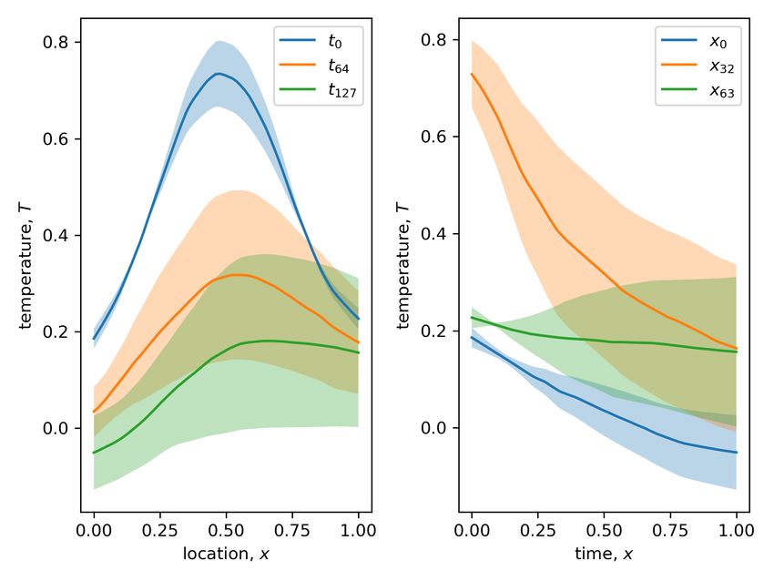
Published at ICLR 2021 Workshop on AI for Modeling Oceans and Climate Change
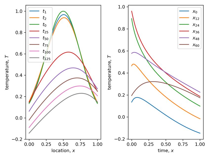
Figure 1: Local advection diffusion equation. The local advection diffusion equation simulates how the initial
temperature profile, T (t = 0, z) (green), is distributed over time. We can observe that the positive diffusivity,
κ > 0, flattens the temperature curve (left) and the vertical velocity, w > 0, shifts the curve to the right over
time.
While most work in physics-informed deep learning has focused on deterministic methods, recent
methods explore the expansion to stochastic differential equations (Zhang et al., 2019; Dandekar
et al., 2021; Yang et al., 2020; Zhu et al., 2019; Liu Yang, 2020). In particular, Zhang et al.
(2019) achieves lightweight surrogate models for parameter estimation and uncertainty propaga-
tion by combining physics-informed neural networks (Raissi et al., 2019) with arbitrary polynomial
chaos (Wan & Karniadakis, 2006). We use the simpler polynomial chaos expansion (Smith, 2013)
instead of arbitrary polynomial chaos expansion, and focus on the task of uncertainty propagation
in (Zhang et al., 2019). Further, we are the first in applying the combination of polynomial chaos
and neural networks to the stochastic local advection-diffusion equation (ADE). Methods of un-
certainty quantification have extensively been demonstrated on the local ADE (Smith, 2013); the
advantage of neural networks is the ability to estimate PCE coefficients in high-dimensional spaces.
The local ADE, also called horizontally averaged Boussinesq equation, is more challenging than the
1D stochastic diffusion equation from (Zhang et al., 2019) and illustrates the application to ocean
modeling.
In summary our work contributes, PCE-PINNs, the first method for fast uncertainty propagation of
parameter uncertainties with physics-informed neural networks in ocean modeling.
2 A PPROACH
We are defining the initial value problem of solving the stochastic partial differential equation,
Nz [T (t, z; ω); κ(z; ω)] = 0, t, z ∈ D, ω ∈ Ω,
B.C.: Bt,z [T (t = 0, z; ω)] = 0,
with spatial domain, Dz , temporal domain, Dt , random space, Ω, domain boundary, Γ, nonlinear
operator, N , and Dirichlet boundary conditions, Bt,z .
2.1 D EFINING THE LOCAL ADVECTION - DIFFUSION EQUATION
We are given the local advection-diffusion equation which models the temperature distribution in a
vertical ocean column over time,
δT (t, z; ω) δ δ δT (t, z; ω)
f= + (wT (t, z; ω)) − κ(z; ω) (1)
δt δz δz δz
with height, z ∈ Dz = [0, 1], time, t ∈ Dt = [0, 1], source, f = 0, noise, ω ∈ Ω, temperature,
T : Dt , Dz → R, stochastic diffusivity, κ(z, ω), constant vertical velocity, w = 10.
We assume that the distribution over the diffusivity is known, for example, through data assimilation
or Bayesian parameter estimation. Specifically, the diffusivity is assumed to follow an exponential
Gaussian process (GP) with κ(z; ω) = exp(Yκ (z; ω)). The GP, Yκ (z; ω), is defined by mean,
2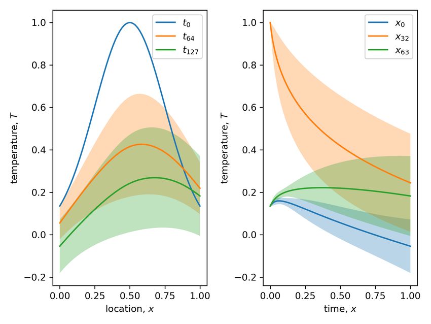
Published at ICLR 2021 Workshop on AI for Modeling Oceans and Climate Change

µYκ = 1000, correlation length, L = 0.3, variance, σYκ = 1.0, exponent, pGP = 1.0, and a
covariance kernel that is similar to the non-smooth Ornstein-Uhlenbeck kernel:

                                                                 1 |z1 − z2 | p
                          CovYκ (z1 , z2 ) = σY2 κ exp(−            (        ) ).                  (2)
                                                                pGP    L

2.2   P OLYNOMIAL CHAOS EXPANSION IN NEURAL NETWORKS

In practice, computing ensembles of differential equations such as in equation (1) for a distribution
of parameter inputs is often computationally prohibitive. Hence, we aim to learn a copy, or fast
surrogate model, of the differential equation solver, T̂ : Dx ×Dz → R, assuming a known parameter
distribution and a set of ground truth solutions, T ∈ T, from the solver.
The polynomial chaos expansion (PCE) approximates arbitrary stochastic functions by a linear
combination of polynomials (Smith, 2013). The polynomials capture the stochasticity by apply-
ing a nonlinear function to typically simple distributions and the coefficients capture the spatio-
temporal dependencies (Smith, 2013). PCE has been widely adopted in computational fluid dynam-
ics (CfD) community, because it offers fast inference time, analytical statistical summaries, such as
C0 = µT , and the theoretical guarantees of polynomials (Smith, 2013). However, the computation
of PCE coefficients, Cα~ (t, z), is analytically complex, because the computation differs among prob-
lems, and computationally expensive, because the computation involves integrals over the random
space (Smith, 2013). Hence, we leverage neural networks to learn the PCE coefficients, Ĉα~ (t, z),
directly from observations of the solution.
The polynomial chaos expansion then approximates the solution as,
                                              |A|
                                              X
                                        ~ =
                              T̂ (t, z; ξ)          Ĉα~ j (t, z)Ψα~ j (ξ1 , ..., ξn )             (3)
                                              j=0

with the NN-based PCE coefficients, Ĉα~ (t, z) ∈ R, the vector of polynomial degrees or multi-index,
~ j ∈ A with j ∈ {0, ..., |A|}, the set of multi-indices, A, the maximum polynomial degree, n, and
α
                              ~ The polynomials are defined by a set of multivariate orthogonal
the set of polynomials, Ψα~ (ξ).
Gaussian-Hermite polynomials,
                                  Ψα~ j (ξ1 , ..., ξn ) = Πni=1 ψαji (ξi ),
                                                       = Πni=1 Heαji (ξi ),                        (4)
                                             with ξi ∼ N (0, 1).
with the one-term (monic) polynomials, ψαji of polynomial degree, αji . We are choosing the ran-
dom vector of each stochastic dimension, i ∈ {0, ..., n}, to be a Gaussian, ξi ∼ N (0, 1) and
use the associated probabilists’ Hermite polynomials, Heαji . The polynomial degrees are given
                                                                         Pn
by the total-degree multi-index set, A = {~         αj ∈ Nn0 : ||~
                                                                 αj ||1 = i=1 αji ≤ n}. For example,
A = {[0, 0], [0, 1], [1, 0], [1, 1], [2, 0], [0, 2]} for n = 2. The number of terms, |A|, is given by,
|A| = (n+n)!
        n!n! .
The neural network (NN) then jointly approximates all PCE coefficients,
                            N NCA (t, z) := ĈA (t, z) : Dt × Dz → R|A| .                          (5)

The NN is trained to approximate PCE coefficients while only using the limited number of measure-
ments, T ∈ R, as target data. The mean-squared error (MSE) loss function for episode, e, and batch
size, B, is defined as:
                                    B
                                  1 X
                  Le (tb , zb ) =     ||Tb − T̂α~ ||22 ,
                                  B
                                     b=1
                                                          |A|
                                                                                                   (6)
                                  B
                                1 X                ~
                                                          X
                              =     ||T (tb , zb ; ξb ) −     Ĉα~ j (tb , zb )Ψα~j (ξ~b )||22 ,
                                B                         j=0
                                     b=1

                                                        3
Published at ICLR 2021 Workshop on AI for Modeling Oceans and Climate Change
(a) Target solution (b) PCE-PINN solution (ours)
Figure 2: PCE-PINNs. Initial results show that the PCE-PINNs in Fig. 2b can approximately match the mean
(line) and standard deviation (shade) of the target solution in Fig. 2a with M SE = 0.0078. Importantly the
approximated standard deviation also captures the growing trend towards the center location (x = 0.5) and
growing time, t = 1.
where the realizations of random vectors, ξ~b ∼ N (0, 1)n are shared between the target and approx-
imated solution. The batch size is chosen to fit one solution sample, B = nt nz with t-grid size, nt ,
and z-grid size, nz .
3 R ESULTS
Figure 2 shows that the PCE-PINNs in Fig. 2b can successfully approximate the mean and stan-
dard deviation of the target solution Fig. 2a. Importantly the explicit formulation as polynomial
chaos expansion allows us to compute the mean and standard deviation without any sampling as a
function of the PCE coefficients, e.g., µT (t, z) = C[ 0, 0, 0](t, z). We can note that the PCE-PINN-
approximated standard deviation captures the growing trend towards the center location (x = 0.5)
and increasing time (t = 1). Quantitative analysis shows that the mean error is, as a sum over the
full spatio-temporal domain, low M SE = 0.0078.
We observe that the PCE-PINNs slightly overestimate the uncertainty of the initial state (blue),
have a marginal positive bias towards the right boundary (x ≈ 1), and have lower curvature during
the initial steps (t ≈ 0). Future work will explore stronger constraints on satisfying the underlying
physics equations and explore a broader choice of neural networks hyperparameters to further reduce
the error.
We used a 2-layer 128-unit fully-connected neural network with ReLu activation. The network was
trained with the ADAM optimizer with learning rate, lr = 0.001, and β = [0.9, 0.999] for E = 15
epochs. The target data was generated with nt = 128 temporal and nz = 64 grid points and
ns = 100 samples of the solved differential equation. The maximum polynomial degree was chosen
to be, n = 2, s.t. the number of PCE coefficients, |A| = 3.
Leveraging neural network-based surrogate models can not only reduce computational complexity
but also storage complexity. Our network contains nw = 2nunits + nlayers n2units + nunits |A| =
33408 weights which occupy as floats nweights 4B ≈ 133kB.
4 D ISCUSSION AND FUTURE WORK
We have demonstrated a novel technique for fast uncertainty propagation with physics-informed
neural networks on the local advection-diffusion equation. The PCE-PINNs uses neural networks
to learn the spatio-temporal coefficients of the polynomial chaos expansion, reducing the analytical
and computational complexity of previous methods. Our method learned a lightweight surrogate
model of the local advection-diffusion equation and successfully quantified the output uncertainties,
given known parameter uncertainties.
We note that our results show room for improvement. Future work will explore stronger constraints
on satisfying the physical laws in (1), e.g., via physics-based regularization terms (Raissi, 2018)
or hard physics-constraints (Beucler et al., 2021). Further, computational resources were limited
during this experiment and future work will further optimize the choice of hyperparameters for the
4Published at ICLR 2021 Workshop on AI for Modeling Oceans and Climate Change
neural network. Lastly, the proposed approach requires computation of a training dataset of solved
differential equation for a set of parameter samples which can quickly become computationally
expensive. Future work, will explore self-supervised learning approaches to enable learned surrogate
models without the use of expensive training data.
ACKNOWLEDGMENTS
The authors greatly appreciate the discussions with Chris Hill, Hannah Munguia-Flores, Brandon
Leshchinskiy, Nicholas Mehrle, Yanni Yuval, Paul O’Gorman, and Youssef Marzouk.
Research was sponsored by the United States Air Force Research Laboratory and the United States
Air Force Artificial Intelligence Accelerator and was accomplished under Cooperative Agreement
Number FA8750-19-2-1000. The views and conclusions contained in this document are those of the
authors and should not be interpreted as representing the official policies, either expressed or im-
plied, of the United States Air Force or the U.S. Government. The U.S. Government is authorized to
reproduce and distribute reprints for Government purposes notwithstanding any copyright notation
herein.
R EFERENCES
David Bau, Jun-Yan Zhu, Hendrik Strobelt, Agata Lapedriza, Bolei Zhou, and Antonio Torralba.
Understanding the role of individual units in a deep neural network. Proceedings of the National
Academy of Sciences, 2020. ISSN 0027-8424.
Tom Beucler, Michael Pritchard, Stephan Rasp, Jordan Ott, Pierre Baldi, and Pierre Gentine. En-
forcing analytic constraints in neural networks emulating physical systems. Phys. Rev. Lett., 126:
098302, Mar 2021.
Noah D. Brenowitz, Tom Beucler, Michael Pritchard, and Christopher S. Bretherton. Interpreting
and stabilizing machine-learning parametrizations of convection. Journal of the Atmospheric
Sciences, 77(12):4357 – 4375, 2020.
Tian Qi Chen, Yulia Rubanova, Jesse Bettencourt, and David K Duvenaud. Neural ordinary dif-
ferential equations. In Advances in Neural Information Processing Systems 31, pp. 6571–6583.
Curran Associates, Inc., 2018.
Raj Dandekar, Karen Chung, Vaibhav Dixit, Mohamed Tarek, Aslan Garcia-Valadez, Krishna Vishal
Vemula, and Chris Rackauckas. Bayesian neural ordinary differential equations, 2021.
O. Fuhrer, T. Chadha, T. Hoefler, G. Kwasniewski, X. Lapillonne, D. Leutwyler, D. Lüthi, C. Osuna,
C. Schär, T. C. Schulthess, and H. Vogt. Near-global climate simulation at 1 km resolution:
establishing a performance baseline on 4888 gpus with cosmo 5.0. Geosci. Model Dev., 11:
1665–1681, 2018.
Luis A. Garcia and Abdalla Shigidi. Using neural networks for parameter estimation in ground
water. Journal of Hydrology, 318(1):215–231, 2006.
Tilmann Gneiting and Adrian E. Raftery. Weather forecasting with ensemble methods. Science, 310
(5746):248–249, 2005.
Samuel Greydanus, Misko Dzamba, and Jason Yosinski. Hamiltonian neural networks. In H. Wal-
lach, H. Larochelle, A. Beygelzimer, F. d Alché-Buc, E. Fox, and R. Garnett (eds.), Advances in
Neural Information Processing Systems 32, pp. 15379–15389. Curran Associates, Inc., 2019.
Anuj Karpatne, William Watkins, Jordan Read, and Vipin Kumar. Physics-guided Neural Networks
(PGNN): An Application in Lake Temperature Modeling. arXiv e-prints, pp. arXiv:1710.11431,
October 2017.
Thorsten Kurth, Sean Treichler, Joshua Romero, Mayur Mudigonda, Nathan Luehr, Everett H.
Phillips, Ankur Mahesh, Michael Matheson, Jack Deslippe, Massimiliano Fatica, Prabhat, and
Michael Houston. Exascale deep learning for climate analytics. Proceedings of the International
Conference for High Performance Computing, Networking, Storage, and Analysis, 51:1–12, 2018.
5Published at ICLR 2021 Workshop on AI for Modeling Oceans and Climate Change
Timothée Lesort, Mathieu Seurin, Xinrui Li, Natalia Dı́az-Rodrı́guez, and David Filliat. Deep un-
supervised state representation learning with robotic priors: a robustness analysis. In 2019 Inter-
national Joint Conference on Neural Networks (IJCNN), pp. 1–8. IEEE, 2019.
George Em Karniadakis Liu Yang, Dongkun Zhang. Physics-Informed Generative Adversarial Net-
works for Stochastic Differential Equations. SIAM Journal on Scientific Computing, 42(1):A292–
A317, 2020.
Zichao Long, Yiping Lu, and Bin Dong. Pde-net 2.0: Learning pdes from data with a numeric-
symbolic hybrid deep network. Journal of Computational Physics, 399:108925, 2019.
B. Lusch, J.N. Kutz, and S.L. Brunton. Deep learning for universal linear embeddings of nonlinear
dynamics. Nat. Commun., 9, 2018.
Björn Lütjens*, Brandon Leshchinskiy*, Christian Requena-Mesa*, Farrukh Chishtie*, Natalia
Dı́az-Rodrı́guez*, Océane Boulais*, Aruna Sankaranarayanan*, Aaron Pi na, Yarin Gal, Chedy
Raı̈ssi, Alexander Lavin, and Dava Newman. Physically-consistent generative adversarial net-
works for coastal flood visualization. arXiv e-prints, 2021. URL https://arxiv.org/
abs/2104.04785. * equal contribution.
Arvind T. Mohan, Nicholas Lubbers, Daniel Livescu, and Michael Chertkov. Embedding hard
physical constraints in neural network coarse-graining of 3d turbulence. ICLR Workshop on AI
for Earth Sciences, 2020.
Christopher Rackauckas, Yingbo Ma, Julius Martensen, Collin Warner, Kirill Zubov, Rohit Supekar,
Dominic Skinner, and Ali Ramadhan. Universal differential equations for scientific machine
learning. ArXiv, abs/2001.04385, 2020.
M. Raissi, P. Perdikaris, and G.E. Karniadakis. Physics-informed neural networks: A deep learn-
ing framework for solving forward and inverse problems involving nonlinear partial differential
equations. Journal of Computational Physics, 378:686 – 707, 2019.
Maziar Raissi. Deep hidden physics models: Deep learning of nonlinear partial differential equa-
tions. Journal of Machine Learning Research, 19(25):1–24, 2018.
Stephan Rasp, Michael S. Pritchard, and Pierre Gentine. Deep learning to represent subgrid pro-
cesses in climate models. Proceedings of the National Academy of Sciences, 115(39):9684–9689,
2018.
Markus Reichstein, Gustau Camps-Valls, Bjorn Stevens, Martin Jung, Joachim Denzler, Nuno Car-
valhais, and Prabhat. Deep learning and process understanding for data-driven earth system sci-
ence. Nature, 566:195 – 204, 2019.
Jakob Runge, Sebastian Bathiany, Erik Bollt, Gustau Camps-Valls, Dim Coumou, Ethan Deyle,
Clark Glymour, Marlene Kretschmer, Miguel D. Mahecha, Jordi Muñoz-Marı́, Egbert H. van
Nes, Jonas Peters, Rick Quax, Markus Reichstein, Marten Scheffer, Bernhard Schölkopf, Peter
Spirtes, George Sugihara, Jie Sun, Kun Zhang, and Jakob Zscheischler. Inferring causation from
time series in earth system sciences. Nature Communications, 10(2553), 2019.
Ralph C. Smith. Uncertainty quantification: Theory, implementation, and applications. In Compu-
tational science and engineering, pp. 382. SIAM, 2013.
J. Nathan Kutz Steven L. Brunton. Data-Driven Science and Engineering: Machine Learning,
Dynamical Systems, and Control. Cambridge University Press, February 2019.
Xiaoliang Wan and George Em Karniadakis. Multi-element generalized polynomial chaos for arbi-
trary probability measures. SIAM J. Sci. Comput., 28(3):901–928, March 2006.
Yibo Yang, Mohamed Aziz Bhouri, and Paris Perdikaris. Bayesian differential programming for ro-
bust systems identification under uncertainty. Proceedings of the Royal Society A: Mathematical,
Physical and Engineering Sciences, 476(2243), 2020.
Janni Yuval and Paul A. O’Gorman. Stable machine-learning parameterization of subgrid processes
for climate modeling at a range of resolutions. Nature Communications, 11, 2020.
6Published at ICLR 2021 Workshop on AI for Modeling Oceans and Climate Change
Janni Yuval, Paul A. O’Gorman, and Chris N. Hill. Use of neural networks for stable, accurate and
physically consistent parameterization of subgrid atmospheric processes with good performance
at reduced precision. Geophysical Research Letter, 48:e2020GL091363, 2021.
Dongkun Zhang, Lu Lu, Ling Guo, and George Em Karniadakis. Quantifying total uncertainty in
physics-informed neural networks for solving forward and inverse stochastic problems. Journal
of Computational Physics, 397:108850, 2019.
Yinhao Zhu, Nicholas Zabaras, Phaedon-Stelios Koutsourelakis, and Paris Perdikaris. Physics-
constrained deep learning for high-dimensional surrogate modeling and uncertainty quantification
without labeled data. Journal of Computational Physics, 394:56 – 81, 2019.
7You can also read