Pizza sauce spread classification using colour vision and support vector machines
←
→
Page content transcription
If your browser does not render page correctly, please read the page content below
Journal of Food Engineering 66 (2005) 137–145
                                                                                                                www.elsevier.com/locate/jfoodeng

                  Pizza sauce spread classification using colour vision
                             and support vector machines
                                                Cheng-Jin Du, Da-Wen Sun                        *

FRCFT Group, Department of Biosystems Engineering, University College Dublin, National University of Ireland, Earlsfort Terrace, Dublin 2, Ireland
                                                Received 1 October 2003; accepted 1 March 2004

Abstract
   An automated classification system of pizza sauce spread using colour vision and support vector machine (SVM) was developed.
To characterise pizza sauce spread with low dimensional colour features, a sequence of image processing algorithms was developed.
After image segmentation from the background, the segmented image was transformed from red, green, and blue (RGB) colour
space to hue, saturation, and value (HSV) colour space. Then a vector quantifier was designed to quantify the HS (hue and sat-
uration) space to 256-dimension, and the quantified colour features of pizza sauce spread were represented by colour histogram.
Finally, principal component analysis (PCA) was applied to reduce the 256-dimensional vectors to 30-dimensional vectors. With the
30-dimensional vectors as the input, SVM classifiers were used for classification of pizza sauce spread. It was found that the
polynomial SVM classifiers resulted in the best classification accuracy with 96.67% on the test experiments.
 2004 Elsevier Ltd. All rights reserved.

Keywords: Classification; Colour; Computer vision; Image processing; Machine vision; Principal component analysis; PCA; Pizza; Pizza sauce; Pizza
topping; Support vector machine, SVM; Vector quantification

1. Introduction                                                             ranges ½220; 14, ½0; 125 and ½0; 200, respectively, seg-
                                                                            mentation of pizza sauce from pizza base was achieved.
   The sauce is everything and can be a signature part of                   Finally, segmentation of the light zones of pizza sauce
the pizza (Burg, 1998). Therefore, the quality of pizza                     was accomplished by setting the HSI values as follows:
sauce spread is an influential factor while evaluating the                   ½2; 14, ½53; 125 and ½106; 200, respectively. The most
whole quality of a pizza. In the pizza industry, the                        disadvantage of the method is that it is likely to become
quality evaluation of pizza sauce spread is still per-                      tuned to one type of image (e.g., a specific sensor, scene
formed manually by trained inspectors, which is tedious,                    setting, illumination, and so on), which limited its
laborious, and costly, and is easily influenced by physi-                    applicability. The performance of the algorithm de-
ological factors, thus inducing subjective and incon-                       grades significantly when the colour and the intensity of
sistent evaluation results. Increased popularity and                        the illuminant are changed.
consumption of pizzas have necessitated the automated                           Image analysis techniques have been used increas-
quality evaluation of pizza sauce spread. Sun and                           ingly for food quality evaluation over the past decades
Brosnan (2003a) analysed images of pizza sauce spread                       (Brosnan & Sun, 2004; Kavdir & Guyer, 2002; Park &
based on simple thresholding segmentation that in-                          Chen, 2000; Sun, 2000, 2004; Sun & Brosnan, 2003b; Sun
cluded three steps. Firstly the whole pizza image was                       & Du, 2004; Wang & Sun, 2001). In image analysis for
segmented from the white background using the red,                          food products, colour is an influential attribute of visual
green, and blue (RGB) model. Then by setting the hue,                       information and powerful descriptor for measurement.
saturation, and intensity (HSI) values in the following                     Colour vision offers a tremendous amount of spatial
                                                                            resolution that can be used to quantify the colour dis-
                                                                            tribution of ingredients. Colour features of an object can
  *                                                                         be extracted by examining every pixel within the object
    Corresponding author. Tel.: +353-1-7165528; fax: +353-1-
4752119.
                                                                            boundaries and have proven successful for the objective
   E-mail address: dawen.sun@ucd.ie (D.-W. Sun).                            measurement of many types of food products with
   URL: http://www.ucd.ie/refrig.                                           applications ranging from fruit, grain, meat, to vegetable
0260-8774/$ - see front matter  2004 Elsevier Ltd. All rights reserved.
doi:10.1016/j.jfoodeng.2004.03.011
138 C.-J. Du, D.-W. Sun / Journal of Food Engineering 66 (2005) 137–145
Nomenclature
~
v assumed vector of two-dimensional HS col- h hue component of HSV colour space
our space i, m, n index variable
~
ui eigenvector of the covariance matrix k kernel function
!
cy i new colour feature vector l number of pizza sauce spread samples
uðÞ
~ non-linear transformation M assumed number of colours
~
w normal to the hyperplane nb normalised blue component of RGB colour
!
cx i quantified colour feature vectors space
~
c two-dimensional code-vector ng normalised green component of RGB colour
r sigma term of Gaussian radial basis function space
kernels nr normalised red component of RGB colour
ni nonnegative slack variable space
ai coefficient obtained by solving a convex P probability distribution function
quadratic programming problem Q vector quantifier
ki eigenvalue of the covariance matrix R partitioned region of the HS space
~ xi , ~
x, ~ xj input vector RS set of 256 regions
b bias term s saturation component of HSV colour space
C parameter used to penalise variables ni T transformation matrix
CM covariance matrix v value component of HSV colour space
CS set of 256 colours as the codebook VS assumed vector set of two-dimensional HS
d degree of polynomial kernels colour space
f classification function yi class of acceptable or unacceptable quality
H high dimensional feature space level
(Daley & Thompson, 1992; Jahns, Nielsen, & Paul, 2001; space, and then classifies the data by the maximal margin
Leemans, Magein, & Destain, 1998; Ruan et al., 2001). hyperplanes. Moreover, SVM is capable of learning in
Among the applications, one would expect most appli- high-dimensional feature space with fewer training data.
cations to be based on RGB colour space (Ahmad, Reid, Recently, SVM has been successfully applied to numer-
Paulsen, & Sinclair, 1999; Lu, Tan, Shatadal, & Gerrard, ous classification problems, such as electronic nose data
2000) and HSI colour space (Sun & Brosnan, 2003a; Tao, (Pardo & Sberveglieri, 2002; Trihaas & Bothe, 2002) and
Heinemann, Vargheses, Morrow, & Sommer, 1995). bakery process data (Rousu et al., 2003).
However, L a b colour space has also been used for In this paper, a hybrid image processing algorithm was
colour features extraction (Vizhanyo & Felfoldi, 2000). firstly developed to segment the pizza sauce spread from
Classification identifies objects by classifying them the background. Then the RGB colour space was trans-
into one of the finite sets of classes, which involves formed to hue, saturation and value (HSV) colour space,
comparing the measured features of a new object with and the image was represented by hue and saturation
those of a known object or other known criteria and (HS) colour components to ensure illumination indepen-
determining whether the new object belongs to a par- dence. An efficient colour quantification method was
ticular category of objects. A wide variety of approaches presented to characterise the colour contents in the images
have been taken towards this task in the food quality of pizza sauce spread, which were represented by colour
evaluation. They have a common objective that is to histogram. After that, principal component analysis
simulate a human decision-maker’s behaviour. Support (PCA) was applied to reduce the dimensionality of the
vector machine (SVM) is a state-of-the-art classification colour feature vectors, and finally, the SVM classifica-
technique, which has a good theoretical foundation in tion techniques were employed for grading pizza sauce
statistical learning theory (Vapnik, 1998). SVM fixes the spread.
classification decision function based on structural risk
minimisation instead of the minimisation of the mis-
classification on the training set to avoid overfitting 2. Materials and methods
problem. It performs binary classification problem by
finding maximal margin hyperplanes in terms of a subset 2.1. Computer vision system
of the input data (support vectors) between different
classes. If the input data are not linearly separable, SVM The samples of pizza sauce spread were provided by
firstly maps the data into a high dimensional feature Green Isle Foods (Naas, Ireland), which were categor-C.-J. Du, D.-W. Sun / Journal of Food Engineering 66 (2005) 137–145 139
ised into five quality levels by the qualified inspection Edge detection
personnel in the company, i.e., reject underwipe,
acceptable underwipe, even spread, acceptable overwipe
and reject overwipe. The image acquisition system used Morphological
dilation
in this study consists of a Dell Workstation 400 equip-
ped with an IC-RGB frame grabber (Imaging Technol-
ogy, US), and a high quality 3-CCD Sony XC-003P Flood filling
camera. The images of pizza sauce spread were captured
under two fluorescent lamps with plastic light diffusers.
Image smoothing
The overall sequence of digital image processing algo-
rithms for classification of pizza sauce spread was
presented in Fig. 1. Mask operation
Fig. 2. The block diagram of image segmentation algorithm.
2.2. Image segmentation
To partition the image of pizza sauce spread from the of image segmentation algorithm sequences was shown
background, a gradient-based segmentation approach in Fig. 2.
was developed, which includes five steps, i.e., edge
detection, morphological dilation, flood filling, image
2.3. Colour space transformation
smoothing and mask operation. For the pizza image
that differs greatly in contrast from the background, the
Since colour is invariant with respect to camera po-
Sobel operator (Sobel, 1970) was applied to detect the
sition and pizza orientation, it is one of the most sig-
edge of pizza. The threshold value employed by Sobel
nificant features for pizza measurement. The images of
operator for edge detection was determined using Otsu’s
pizza sauce spread were taken by the CCD camera and
method (Otsu, 1979). To eliminate the gaps in the edges,
saved in the three-dimensional RGB colour space.
morphological dilation was implemented to the edge
Unfortunately, the RGB colour space used in computer
image. Then a flood filling operation (Soille, 1999) was
graphics is device dependent, which is designed for
performed to fill the holes in the image and a disk
specific devices, e.g. cathode-ray tube (CRT) display.
structure element was used to smooth the object by
Therefore, the RGB space has no accurate definition for
eroding the image twice. Finally, mask operation was
a human observer, where the proximity of colours in the
applied to the original image to obtain the region of
space does not indicate colour similarity in perception.
interest, i.e., the pizza sauce spread. The block diagram
Colour space transformations are effective means for
distinguishing colour images, which is an operation on
the original colour space to produce a new transformed
Image acquisition space. Linear transformation is the simplest method for
colour conversion from the RGB space to others. Sev-
eral linear transformations are used for transmitting
Image segmentation
videos and representing colour images. For example,
YUV (standard colour space used in European TVs,
Colour space where Y is linked to the component of luminance, and U
transformation and V are linked to the components of chrominance)
and i1i2i3 (Ohta, Kanade, & Sakai, 1980) are obtained
by linear transformation through simple matrix multi-
Colour
quantification
plications. Other colour space transformations are more
complex, such as HSV and L a b , which are generated
by non-linear transformations.
Dimensionality Compared to the other colour spaces, HSV is an
reduction by principal
intuitive colour space, which is a user-oriented colour
component analysis
system based on the artist’s idea of tint, shade and tone.
HSV separates colour into three components, i.e., hue
Classification using (H), saturation (S) and value (V). H distinguishes among
support vector the perceived colours, such as red, yellow, green and
machines
blue. S refers to how far a colour is from a grey of equal
Fig. 1. The overall sequence of digital image processing algorithms for intensity, and V represents the brightness of a reflecting
classification of pizza sauce spread. object. For efficient classification of pizza sauce spread,140 C.-J. Du, D.-W. Sun / Journal of Food Engineering 66 (2005) 137–145
the RGB colour space was transformed to HSV space. The colour histogram method is one of the simplest
Given the normalised r; g; b 2 ½0; . . . ; 1, the transfor- and most popular approaches to characterise colour
mation to HSV is achieved by the following equations: information in the images. Using the 256-colour quan-
tified HS space, the distribution of colour content in the
v ¼ maxðnr; ng; nbÞ ð1Þ
image of pizza sauce spread was represented by a colour
v minðnr; ng; nbÞ histogram. Column III in Fig. 3 showed five examples of
s¼ ð2Þ
v quantified colour histogram of pizza sauce spread. The
Let abscissa is the index of code-vector n and the ordinate
v nr is the frequency of occurrence.
tr ¼ ;
v minðnr; ng; nbÞ
v ng 2.5. Dimensionality reduction by principal component
tg ¼ ; analysis
v minðnr; ng; nbÞ
v nb In real implementation, the quantified 256-dimen-
tb ¼ ;
v minðnr; ng; nbÞ sional vectors are still too large to allow fast and accu-
then rate classification. The large feature vectors will increase
8 the complexity of the classifier and the classification
>
> 5 þ tb if nr ¼ maxðnr; ng; nbÞ and ng ¼ minðnr; ng; nbÞ
>
> error. PCA is one of the powerful techniques for
>
> 1 tg if nr ¼ maxðnr; ng; nbÞ and ng 6¼ minðnr; ng; nbÞ
< dimensionality reduction (Calvo, Partridge, & Jabri,
1 þ tr if ng ¼ maxðnr; ng; nbÞ and nb ¼ minðnr; ng; nbÞ
6h ¼
> 3 tb if ng ¼ maxðnr; ng; nbÞ and nb 6¼ minðnr; ng; nbÞ
> 1998), which transforms original feature vectors from
>
>
>
> 3 þ tg if nb ¼ maxðnr; ng; nbÞ and nr ¼ minðnr; ng; nbÞ large space to a small subspace with lower dimensions.
:
5 tr otherwise The basic approach of PCA is first to compute the
ð3Þ covariance matrix (CM) of the quantified 256-dimen-
where h; s; v 2 ½0; . . . ; 1. sional vectors. The eigenvalue ki and eigenvector ~ ui of
the covariance matrix (CM) can be obtained by solving
2.4. Colour quantification the eigenstructure decomposition CM~ ui ¼ ki~ui . In prac-
tice, there are two ways to compute the eigenvalues and
Generally, the HSV colour space is discretised to 256 eigenvectors: singular value decomposition (SVD) and
levels at each channel, which yields a very large number regular eigen-computation (Zhao, Chellappa, & Krish-
of colours (256 · 256 · 256). In order to limit the naswamy, 1998). Taken the eigenvectors ~ ui as its rows, a
dimensionality of the colour features of the pizza sauce transformation matrix (T ) is formed. The new colour
spread, the colour space must be reduced and quantified feature vectors ! cy i are obtained by ! cy i ¼ T !cx i , which
into a smaller number of colours, which was realised by maps the quantified 256-dimensional vectors to a smal-
the following three steps. Firstly, to reduce the effect of ler vectors.
illumination on the system, the value component (V ) The first principal component accounts for the most
was not used for colour features extraction of pizza significant characteristic of the original data with the
sauce spread. Then, a vector quantifier (Gray, 1984) was maximum variance. Each succeeding component ac-
designed to quantify the remaining two-dimensional counts for less significant characteristic with as much of
space, i.e., hue and saturation. Finally, colour histogram the remaining variability as possible. Practically, the last
was employed to represent the distribution of colour few principal components can be truncated from the
features in the image of pizza sauce spread. back of the transformation matrix. These principal
After ignoring the value component, the two-dimen- components correspond to useless characteristics that
sional HS space was assumed to consist of MðM 256Þ are essentially noise.
colours: VS ¼ f~ v1 ;~ vM g, where the vectors were
v2 ; . . . ;~
two-dimensional, i.e., ~ vm ¼ ðvm;1 ; vm;2 Þ, m ¼ 1; 2; . . . ; M. 2.6. Classification using SVM
The hue and saturation components were quantified into
16 intervals respectively to produce a set of 256 colours The classification of pizza sauce spread into accept-
as the codebook: CS ¼ f~ c1 ;~ c256 g, where the code-
c2 ; . . . ;~ able and unacceptable quality levels can be considered
vectors were two-dimensional, i.e., ~ cn ¼ ðcn;1 ; cn;2 Þ, as a binary categorisation problem. Suppose there are l
n ¼ 1; 2; . . . ; 256. In this way, the HS space was parti- samples of pizza sauce spread in the training data, and
tioned into 256 regions: RS ¼ fR1 ; R2 ; . . . ; R256 g. Thus, a each sample is denoted by a vector ~xi , which represents
vector quantifier (Q) was generated, which mapped the the colour features of the pizza sauce spread. The clas-
vector set VS containing M inputs into a finite set CS sification of pizza sauce spread can be described as the
containing 256 outputs: Qð~ vm Þ ¼ ~ cn , if ~vm 2 Rn . The task of finding a classification function f : ~ xi ! yi ; yi 2
aforementioned quantification yielded a collection of 256 f1; þ1g using training data. Subsequently, the classi-
distinct colours in HS space. fication function f is used to classify the unseen testC.-J. Du, D.-W. Sun / Journal of Food Engineering 66 (2005) 137–145 141
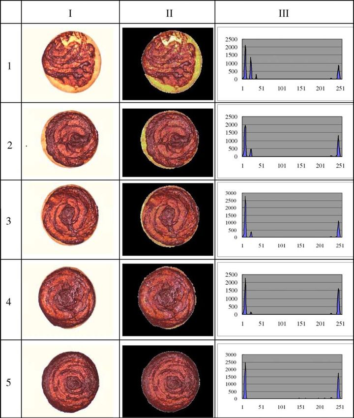
Fig. 3. Results of the image segmentation and colour features extraction algorithms. Column I: original images of the pizza sauces; column II:
segmentation results; column III: colour histograms of the segmented images. Row 1: reject underwipe; row 2: acceptable underwipe; row 3: even
spread; row 4: acceptable overwipe; row 5: reject overwipe.
1 T
data. If f ð~
xi Þ > 0, the input vector ~
xi is assigned to the 2
~ w,
w ~ subject to constraints (5), which is a convex
class yi ¼ þ1, i.e., the acceptable quality level, otherwise quadratic programming problem.
to the class yi ¼ 1, i.e., the unacceptable quality level. For the linearly non-separable case, constraints (5)
For the linearly separable training vectors, the clas- are relaxed by introducing a new set of nonnegative
sification function f has the following form: slack variables fni ji ¼ 1; 2; . . . ; lg as the measurement of
violation of the constraints (Vapnik, 1998) as follows:
f ð~ wT~
xÞ ¼ sgnð~ x þ bÞ ð4Þ
wT~
yi ð~ xi þ bÞ P 1 ni i ¼ 1; 2; . . . ; l ð6Þ
where ~
w is the normal to the hyperplane and b is a bias
term, which should satisfy the following conditions: The optimal hyperplane is the one that minimises the
following formula:
wT~
yi ð~ xi þ bÞ P 1 i ¼ 1; 2; . . . ; l ð5Þ
1 T Xl
The SVM is trying to find the optimal separating ~ wþC
w ~ ni ð7Þ
2 i¼1
hyperplane that maximises the margin between positive
and negative samples. The margin is 2=k~wk, thus the where C is a parameter used to penalise variables ni ,
optimal separating hyperplane is the one minimising subject to constraints (6).142 C.-J. Du, D.-W. Sun / Journal of Food Engineering 66 (2005) 137–145
For nonlinearly separable case, the training vectors ~
xi Then, the vector quantifier described in Section 2.4 was
can be mapped into a high dimensional feature space H applied to extract the colour features of the pizza sauce
by a non-linear transformation ~ uðÞ. The training vec- spread. The quantified colour histogram of the five
tors become linearly separable in the feature space H segmented images in the second column of Fig. 3 were
and then separated by the optimal hyperplane described shown in the third column of Fig. 3. It can be observed
as before. In many cases, the dimension of H is infinite, that the histograms differ sequentially from Fig. 3-III1
which makes it difficult to work with ~ uðÞ explicitly. (reject underwipe) to Fig. 3-III5 (reject overwipe) with
Since the training algorithm only involves inner prod- the sauce spread on the pizza base increasing. In Fig. 3-
ucts in H , a kernel function kð~ yÞ is used to solve the
x;~ III1, there are four big peaks (greater than 100), which
problem, which defines the inner product in H : are located in the following ranges ½1; 13, ½17; 27,
kð~ yÞ ¼ h~
x;~ uð~ uð~
xÞ; ~ yÞi ð8Þ ½33; 39 and ½241; 251, respectively. However, in Fig. 3-
III5, there are only two big peaks located in the ranges
Polynomial kernels and Gaussian radial basis function ½1; 13 and ½242; 251, respectively. Fig. 3-III1 (reject
(RBF) kernels are usually applied in practice and are underwipe) and Fig. 3-III5 (reject overwipe) are unac-
defined as: ceptable levels for too little sauce or too much sauce.
kð~ yÞ ¼ ð~
x;~ y þ bÞd
x~ ð9Þ Contrastively, there are three big peaks in Fig. 3-III2,
III3 and III4, respectively, which are all acceptable
2 2
kð~ yÞ ¼ expðk~
x;~ x ~
yk =2r Þ ð10Þ levels, namely acceptable underwipe, even spread, and
acceptable overwipe. The big peak located in the range
where b is the bias term and d is the degree of polyno-
½33; 39 disappears in the three acceptable levels, and the
mial kernels.
big peak located in ½17; 27 decreases gradually from the
The classification function then has the following
form in terms of kernels: acceptable underwipe to the acceptable overwipe. Based
" # on the colour histogram, it is not difficult to classify the
X
l
five images into acceptable and unacceptable levels. The
f ð~
xÞ ¼ sgn yi ai kð~ xÞ þ b
xi ;~ ð11Þ three images of acceptable levels have three big peaks,
i¼1
while the other two images of unacceptable levels have
where ai can be obtained by solving a convex quadratic four or two big peaks. The illustrational results indicate
programming problem subject to linear constraints. The that the colour contents in the images of pizza sauce
support vectors are those ~
xi with ai > 0 in Eq. (11). spread can be characterised efficiently by the algorithm
developed.
256-dimensional vectors are still too large to classify
3. Results and discussion accurately with small sample sizes. Meanwhile, it is easy
to find that there are a number of portions of the
In this study, 120 images of pizza sauce spread were quantified colour histogram with zero value. PCA was
captured for classification, including 60 acceptable levels applied to reduce the dimensionality of the colour fea-
(15 acceptable underwipe, 25 even spread and 20 accept- tures. The analysis showed that 99.98% of the total
able overwipe) and 60 unacceptable levels (30 reject un- variation is explained by the first 30 principal compo-
derwipe and 30 reject overwipe). The image segmentation nents. The results were visualised by a scatter plot
algorithm of pizza sauce spread described above was (shown in Fig. 4), where the abscissa corresponds to the
implemented by using Matlab (Mathworks, 1992) under first principal component explained 51.76% of the total
Windows NT 4.0 on a Dell Workstation 400. Five images variation and the ordinate corresponds to the second
of pizza sauce spread were chosen to demonstrate the principal component explained 17.46% of the total
performance of the algorithm as shown in Fig. 3. The first variation. The samples of pizza sauce spread of the
column (I in Fig. 3) shows five original images including unacceptable levels, i.e., reject underwipe and reject
two unacceptable quality levels, i.e., reject underwipe overwipe, were mostly located in the right and left part
(Fig. 3-I1) and reject overwipe (Fig. 3-I5), and three of the plot, respectively. And the samples of pizza sauce
acceptable quality levels, i.e., acceptable underwipe (Fig. spread of the acceptable levels were mostly located in the
3-I2), even spread (Fig. 3-I3), and acceptable overwipe middle part of the plot.
(Fig. 3-I4). The segmentation results of the five original Sixty images of pizza sauce spread were randomly
images were shown in the second column (II in Fig. 3), selected for training and the remaining 60 images for test.
where the regions of pizza sauce spread were preserved The first 30 principal components of each sample were
well and the background regions were set with black used as input to the classifiers. The SvmFu (Ryan, 2002)
colour. Based on visual judgement, it can be seen that implementation of SVMs was used for classification of
the segmentation is satisfactory. pizza sauces in all experiments. Besides a linear SVM
After that, the segmented image was converted from classifier, polynomial classifiers and RBF classifiers were
RGB colour space to HSV colour space by Eqs. (1)–(3). trained and tested using the kernels defined in Eqs. (9)C.-J. Du, D.-W. Sun / Journal of Food Engineering 66 (2005) 137–145 143
combinations of bias b and degree d. The polynomial
SVM classifiers ð1; 3Þ, ð1; 4Þ, ð2; 2Þ, ð2; 3Þ, ð2; 4Þ, ð2; 5Þ,
and ð2; 6Þ achieved the best classification accuracy of
96.67% on the test experiments. In fact, the polynomial
SVM classifiers with d ¼ 1 are linear SVM classifiers,
which performed worse than any other classifiers with
only 60.00% accuracy. Fig. 5 illustrates visually the use of
three SVM classifiers for classification of samples of
pizza sauce spread characterised by the first two princi-
pal components. The decision boundaries of a RBF, a
polynomial and a linear SVM classifier were demon-
strated by the contours plotted in different type of line.
As shown in Fig. 5, it was impossible to separate the data
set linearly, which was the reason why only 60.00%
accuracy was achieved by the linear SVM classifier.
Fig. 4. PCA plot of the first two principal components.
and (10), respectively. A range of parameters for the
polynomial and RBF SVM classifiers were selected to
eliminate any biased performance of the SVMs that may
be caused by inappropriate choice of parameters. The
parameters of polynomial SVM were the combinations
of bias b and degree d, with b 2 f0; 1; 2; 3; 4; 5; 6g, and
d 2 f1; 2; 3; 4; 5g. The values r 2 f0:2; 0:5; 0:8; 1:0; 1:2;
1:5; 2:0; 2:5g were selected for the RBF SVM classifiers.
The penalty parameter C in Eq. (7) was set as the default
value 1.0 by the SvmFu algorithm (Ryan, 2002).
The classification results with linear SVM and RBF
SVM classifiers are listed in Table 1. On the test experi-
ments, the RBF kernel with r ¼ 0:5 resulted in the best
classification rate of 95.00%. Table 2 shows the classifi-
cation results of the polynomial SVM with different Fig. 5. The illustration of three SVM classifiers.
Table 1
The classification results with linear SVM and RBF SVM classifiers
Classifiers Linear SVM RBF SVM
0.2 0.5 0.8 1.0 1.2 1.5 2.0 2.5
Rate (%) 60.00 70.00 95.00 91.67 90.00 91.67 85.00 66.67 68.33
Table 2
The classification results (%) of polynomial SVM with different combinations of bias b and degree d
Bias b Degree d
1 2 3 4 5 6
0 60.00 91.67 63.33 88.33 61.67 68.33
1 60.00 93.33 96.67 96.67 95.00 68.33
2 60.00 96.67 93.33 95.00 95.00 68.33
3 60.00 96.67 93.33 95.00 95.00 68.33
4 60.00 96.67 93.33 95.00 95.00 68.33
5 60.00 96.67 91.67 95.00 95.00 68.33
6 60.00 96.67 91.67 95.00 95.00 68.33144 C.-J. Du, D.-W. Sun / Journal of Food Engineering 66 (2005) 137–145
The decision boundaries of the RBF SVM classifier and References
the polynomial SVM classifier can separate the data set
with comparative error. Therefore, the performance of Ahmad, I. S., Reid, J. F., Paulsen, M. R., & Sinclair, J. B. (1999).
the RBF SVM classifier was comparable with the poly- Color classifier for symptomatic soybean seeds using image
processing. Plant Disease, 83(4), 320–327.
nomial SVM classifier as shown in Tables 1 and 2. Brosnan, T., & Sun, D.-W. (2004). Improving quality inspection of
Although the component V was eliminated to reduce food products by computer vision––a review. Journal of Food
the effect of illumination on the developed computer Engineering, 61(1), 3–16.
vision system, the lighting system is still an important Burg, J. C. (1998). Piecing together the pizza puzzle. Food Product
Design (February), 58.
prerequisite of image acquisition for quality evaluation
Calvo, R. A., Partridge, M. G., & Jabri, M. A. (1998). A comparative
of pizza sauce spread. Fortunately, the lighting hard- study of principal component analysis techniques. In Proceedings
ware used is common and readily available for appli- of the ninth australian conference on neural networks, Brisbane,
cation. In a real inspection task where the illumination QLD.
is changeable, the new classifier can be obtained by Crammer, K., & Singer, Y. (2001). On the algorithmic implementation
training with samples captured under new lighting of multiclass kernel-based vector machines. Journal of Machine
Learning Research, 2, 265–292.
conditions. Daley, W. D., & Thompson, J. C. (1992). Color machine vision for
In practice, binary classification of the pizza sauce meat inspection. In Food processing automation II––proceedings of
spread can satisfy the general requirement of industrial the FPAC conference, ASAE, St. Joseph, Michigan, p. 230.
applications. However, it seems a little arbitrary and still Gray, R. M. (1984). Vector quantization. IEEE ASSP Magazine, 4–29.
cannot satisfy the requirement of multi-classification. Jahns, G., Nielsen, H. M., & Paul, W. (2001). Measuring image
analysis attributes and modelling fuzzy consumer aspects for
Although SVM is originally developed for binary clas- tomato quality grading. Computers and Electronics in Agriculture,
sification, several SVM algorithms have been developed 31, 17–29.
for handling multi-classification problem. One approach Kavdir, I., & Guyer, D. E. (2002). Apple sorting using artificial neural
is by using a combination of several binary SVM clas- networks and spectral imaging. Transactions of the ASAE, 45(6),
1995–2005.
sifiers, such as one-versus-all (Vapnik, 1998), one-ver-
Kreßel, U. H.-G. (1999). Pairwise classification and support vector
sus-one (Kreßel, 1999), and Directed Acyclic Graph machines. In B. Sch€ olkopf, C. J. C. Burges, & A. J. Smola (Eds.),
(DAG) SVM (Platt, Cristianini, & Shawe-Taylor, 2000), Advances in kernel methods: Support vector learning (pp. 255–268).
while the other is by directly using a single optimisation Cambridge, MA: MIT Press.
formulation (Crammer & Singer, 2001). Our future re- Leemans, V., Magein, H., & Destain, M. F. (1998). Defects segmen-
search will involve in dealing with the multi-classifica- tation on ‘Golden Delicious’ apples by using colour machine
vision. Computers and Electronics in Agriculture, 20, 117–130.
tion problem of pizza sauce spread using SVM in details. Lu, J., Tan, J., Shatadal, P., & Gerrard, D. E. (2000). Evaluation of
pork color by using computer vision. Meat Science, 56, 57–60.
Mathworks (1992). Matlab Reference Guide. The MathWorks, Inc.,
4. Conclusions Natick, MA, USA.
Ohta, Y. I., Kanade, T., & Sakai, T. (1980). Color information for
The results presented here have demonstrated the region segmentation. Computer Graphics and Image Processing, 13,
222–241.
ability of the approach based on colour vision and
Otsu, N. (1979). A threshold selection method from gray-level
support vector machine to classify pizza sauce spread. histograms. IEEE Transactions on Systems, Man, and Cybernetics,
Being a user-oriented colour space, HSV was employed 9(1), 62–66.
and the component V was eliminated to reduce the effect Pardo, M., & Sberveglieri, G. (2002). Support vector machines for the
of illumination. The vector quantification and PCA classification of electronic nose data. In Proceedings of the 8th
international symposium on chemometrics in analytical chemistry,
techniques successfully reduced the dimensionality of
Seattle, USA.
colour features of pizza sauce spread obtained from the Park, B., & Chen, Y. R. (2000). Real-time dual-wavelength image
remaining HS space. With the first 30 principal com- processing for poultry safety inspection. Journal of Food Process
ponents as the input, an overall accuracy of 96.67% was Engineering, 23(5), 329–351.
achieved by the polynomial SVM classifiers ð1; 3Þ, ð1; 4Þ, Platt, J. C., Cristianini, N., & Shawe-Taylor, J. (2000). Large margin
DAGs for multiclass classification. Advances in Neural Information
ð2; 2Þ, ð2; 3Þ, ð2; 4Þ, ð2; 5Þ, and ð2; 6Þ, and 95.00% accu-
Processing Systems, 12, 547–553.
racy was obtained using the RBF SVM classifier with Rousu, J., Flander, L., Suutarinen, M., Autio, K., Kontkanen, P., &
r ¼ 0:5. Rantanen, A. (2003). Novel computational tools in bakery process
data analysis: a comparative study. Journal of Food Engineering,
57(1), 45–56.
Acknowledgements Ruan, R., Shu, N., Luo, L. Q., Xia, C., Chen, P., Jones, R., Wilcke, W.,
& Morey, R. V. (2001). Estimation of weight percentage of scabby
wheat kernels using an automatic machine vision and neural
The authors wish to acknowledge the financial assis-
network based system. Transactions of the ASAE, 44(4), 983–988.
tance of the Food Institutional Research Measure as Ryan, R. (2002). Everything old is new again: a fresh look at historical
administered by the Irish Department of Agricultural approaches in machine learning. Ph.D. Thesis, Institute of Tech-
and Food, Dublin. nology, Massachusetts, September 2002.C.-J. Du, D.-W. Sun / Journal of Food Engineering 66 (2005) 137–145 145 Sobel, I. (1970). Camera models and machine perception, AIM-21. Tao, Y., Heinemann, P. H., Vargheses, Z., Morrow, C. T., & Sommer, Stanford Artificial Intelligence Lab., Palo Alto, USA. H. J., III (1995). Machine vision for color inspection of potatoes Soille, P. (1999). Morphological image analysis: principles and applica- and apples. Transactions of the ASAE, 38(5), 1555–1561. tions. Germany: Springer-Verlag. Trihaas, J., & Bothe, H.H. (2002). An application of support vector Sun, D.-W. (2000). Inspecting pizza topping percentage and distribu- machines to E-nose data. In Proceedings of the 9th international tion by a computer vision method. Journal of Food Engineering, symposium on olfaction and electronic nose, Rome, Italy. 44(4), 245–249. Vapnik, V. (1998). Statistical learning theory. New York, USA: John Sun, D. -W., (Ed.), (2004). Applications of computer vision in the food Wiley & Sons. industry. Journal of Food Engineering, 61, 1–142 (Special issue). Vizhanyo, T., & Felfoldi, J. (2000). Enhancing colour differences in Sun, D.-W., & Brosnan, T. (2003a). Pizza quality evaluation using images of diseased mushrooms. Computers and Electronics in computer vision––part 1 Pizza base and sauce spread. Journal of Agriculture, 26, 187–198. Food Engineering, 57, 81–89. Wang, H.-H., & Sun, D.-W. (2001). Evaluation of the functional Sun, D.-W., & Brosnan, T. (2003b). Pizza quality evaluation using properties of Cheddar Cheese using a computer vision method. computer vision–– Part 2: Pizza topping analysis. Journal of Food Journal of Food Engineering, 49(1), 49–53. Engineering, 57(1), 91–95. Zhao, W., Chellappa, R., & Krishnaswamy, A. (1998). Discriminant Sun, D.-W., & Du, C. J. (2004). Segmentation of complex food images analysis of principal components for face recognition. In Proceed- by stick growing and merging algorithm. Journal of Food ings of the 3rd international conference on automatic face and gesture Engineering, 61(1), 17–26. recognition (pp. 336–341).
You can also read