Scientific Computing WS 2020/2021 Lecture 1 J urgen Fuhrmann
←
→
Page content transcription
If your browser does not render page correctly, please read the page content below
Scientific Computing WS 2020/2021

Lecture 1

Jürgen Fuhrmann
juergen.fuhrmann@wias-berlin.de

                                    Lecture 1 Slide 1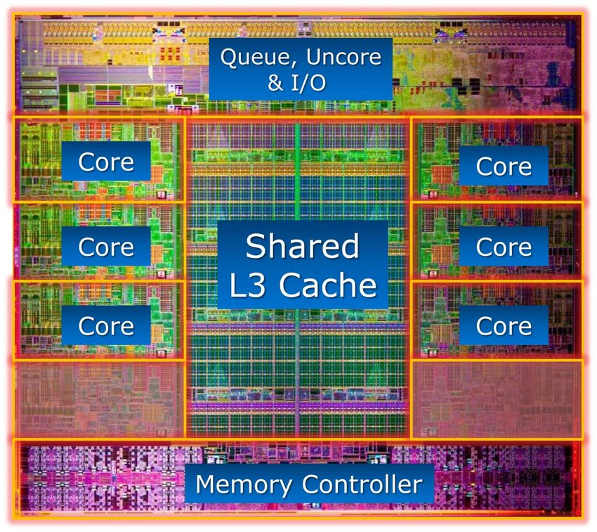
Me

     Name: Dr. Jürgen Fuhrmann (no, not Prof.)
     Affiliation: Weierstrass Institute for Applied Analysis and Stochastics, Berlin
     (WIAS);
     Deputy Head, Numerical Mathematics and Scientific Computing
     Contact: juergen.fuhrmann@wias-berlin.de
     Course homepage:
     https://www.wias-berlin.de/people/fuhrmann/SciComp-WS2021/
     Experience/Field of work:
          Numerical solution of partial differential equations (PDEs)
          Development, investigation, implementation of finite volume discretizations
          for nonlinear systems of PDEs
          Ph.D. on multigrid methods
          Applications: electrochemistry, semiconductor physics, groundwater. . .
          Software development:
               WIAS code pdelib (http://pdelib.org)
               Languages: C, C++, Python, Lua, Fortran, Julia
               Visualization: OpenGL, VTK

                                                                                  Lecture 1 Slide 2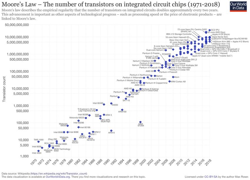
Admin stuff

       Lectures will be recorded
       Slides + Julia notebooks will be available from the course home page
       https://www.wias-berlin.de/people/fuhrmann/SciComp-WS2021/
       Weekly material uploads by Wed night (hopefully)
       Official lecture times: Thu 16-18 and Fri 16-18 will be used for feedback
       sessions with zulip chat and zoom.
       Zoom links will be provided in the chat or per email.
       I will use the email address used for enrolling for all communication, zulip
       invitations etc. Please keep me informed about any changes.
       Please provide missing “Matrikelnummern”
       All code examples and assignments will be in Julia, either as notebooks or
       as Julia files. Things should work on Linux, MacOSX, Windows
       Access to examination
              Attend ≈ 80% of lectures
              Return assignments

                                                                                Lecture 1 Slide 3
Introduction

About computers and (scientific) computing

                                             Lecture 1 Slide 4
There was a time when “computers” were humans

   Harvard Computers, circa 1890
   By Harvard College Observatory - Public Domain
                                                      It was about science – astronomy
   https://commons.wikimedia.org/w/index.php?curid=

   10392913

   Computations of course have been performed since ancient times. One can trace
   back the termin “computer” applied to humans at least until 1613.
   The “Harvard computers” became very famous in this context. Incidently, they
   were mostly female. They predate the NASA human computers of recent movie
   fame.
                                                                                     Lecture 1 Slide 5
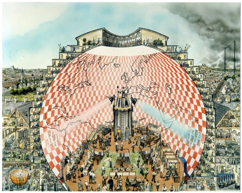
Weather Prediction by Numerical Process

       L.F.Richardson 1922: 64000 human computers sit in rooms attached to a
    transparent cupola, they project their results which are combined by some main
                                computers at the center

                                                                              Lecture 1 Slide 6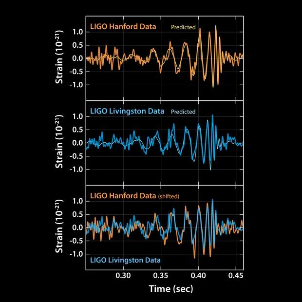
Does this scale ?

              1986 Illustration of L.F. Richardson’s vision by S. Conlin
                                                                           Lecture 1 Slide 7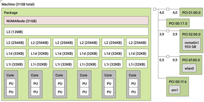
Computing was taken over by machines

        By Max Roser - https://ourworldindata.org/uploads/2019/05/Transistor-Count-over-time-to-2018.png, CC BY-SA 4.0,

                                  https://commons.wikimedia.org/w/index.php?curid=79751151
                                                                                                                          Lecture 1 Slide 8
Computational engineering
Starting points: artillery trajectories, nuclear weapons, rocket design,
weather . . .
Now ubiquitous:
Structural engineering
Car industry
Oil recovery
Semiconductor design
...
Use of well established, verified, well supported commercial codes
Comsol
ANSYS
Eclipse
...
Lecture 1 Slide 9As soon as computing machines became available . . .
. . . Scientists “misused” them to satisfy their curiosity
“. . . Fermi became interested in the development and potentialities of the
electronic computing machines. He held many discussions [. . . ] of the kind of
future problems which could be studied through the use of such machines.”
Fermi,Pasta and Ulam studied particle systems with nonlinear interactions
Calculations were done on the MANIAC-1 computer at Los Alamos
Lecture 1 Slide 10And they still do. . .
SXS, the Simulating eXtreme Spacetimes (SXS) project (http:
//www.black- holes.org)
Caltech/MIT/LIGO Lab
Verification of the detection of gravitational waves by numerical solution of
Einstein’s equations of general relativity using the “Spectral Einstein Code”
Computations significantly contributed to the 2017 Nobel prize in physics
Lecture 1 Slide 11Scientific computing
“The purpose of computing is insight, not numbers.”
(https://en.wikiquote.org/wiki/Richard_Hamming)
Frontiers of Scientific Computing
Insight into complicated phenomena not accessible by other methods
Improvement of models to better fit reality
Improvment of computational methods
Generate testable hypothesis
Support experimentation in other scientific fields
Exploration of new computing capabilities
Prediction, optimization of complex systems
Good scientifc practice
Reproducibility
Sharing of ideas and knowledge
Interdisciplinarity
Numerical Analysis
Computer science
Modeling in specific fields
Lecture 1 Slide 12General approach
Hypothesis
Mathematical model
Algorithm
Code
Result
Possible (probable) involvement of different persons, institutions
It is important to keep interdisciplinarity in mind
Lecture 1 Slide 13Scientific computing tools
Many of them are Open Source
General purpose environments
Matlab
COMSOL
Python + ecosystem
R + ecosystem
Julia
“Classical” computer languages + compilers
Fortran
C, C++
Established special purpose libraries
Linear algebra: LAPACK, BLAS, UMFPACK, Pardiso
Mesh generation: triangle, TetGen, NetGen
Eigenvalue problems: ARPACK
Visualization libraries: VTK
Tools in the “background”
Build systems Make, CMake
Editors + IDEs (emacs, jedit, eclipse, atom, Visual Studio Code)
Debuggers
Version control (svn, git, hg)
Lecture 1 Slide 14Confusio Linguarum
”And the whole land was of one lan-
guage and of one speech. ... And
they said, Go to, let us build us a city
and a tower whose top may reach
unto heaven. ... And the Lord said,
behold, the people is one, and they
have all one language. ... Go to,
let us go down, and there confound
their language that they may not un-
derstand one another’s speech. So
the Lord scattered them abroad from
thence upon the face of all the earth.”
(Daniel 1:1-7)
Lecture 1 Slide 15Once again Hamming
. . . of “Hamming code” and “Hamming distance” fame, who started his carrier
programming in Los Alamos:
“Indeed, one of my major complaints about the computer field is that whereas
Newton could say,”If I have seen a little farther than others, it is because I have
stood on the shoulders of giants,” I am forced to say, “Today we stand on each
other’s feet.” Perhaps the central problem we face in all of computer science is
how we are to get to the situation where we build on top of the work of others
rather than redoing so much of it in a trivially different way. Science is supposed
to be cumulative, not almost endless duplication of the same kind of things.”
(1968)
2020 this is still a problem
Lecture 1 Slide 16Intended aims and topics of this course
Indicate a reasonable path within this labyrinth
Introduction to Julia
Relevant topics from numerical analysis
Focus on partial differential equation (PDE) solution
Solution of large linear systems of equations
Finite elements
Finite volumes
Mesh generation
Linear and nonlinear solvers
Parallelization
Visualization
Lecture 1 Slide 17Hardware aspects
With material from “Introduction to High-Performance Scientific Computing” by
Victor Eijkhout
(http://pages.tacc.utexas.edu/˜eijkhout/istc/istc.html)
Lecture 1 Slide 18von Neumann Architecture
CPU Core Memory (RAM)
Control Data and code stored in the same
ALU
memory ⇒ encoded in the same
way, stored as binary numbers
REG REG REG REG
Instruction cycle:
Instruction decode: determine
Cache
operation and operands
Get operands from memory
Perform operation
Bus
Write results back
Continue with next instruction
Controlled by clock: “heartbeat” of
USB Controller GPU IO Controller CPU
USB IO Mouse Keyboard
Monitor
Traditionally: one instruction per
HDD/SSD clock cycle
Lecture 1 Slide 19Multicore CPU
Modern CPU. From: https://www.hartware.de/review_1411_2.html
Several computational cores on one CPU
Cache: fast intermediate memory for often used operands
Lecture 1 Slide 20Mulicore CPU: this Laptop
Three cache levels
6 Cores with similar pathways to memory
Lecture 1 Slide 21NUMA Architecture: compute server
NUMA: Non
Uniform Memory
Access
Several packages
with 1 NUMA
node each
Each NUMA node
has part of the
system RAM
attached to it.
Lecture 1 Slide 22Modern CPU workings
Multicore parallelism
Multiple floating point units in one core ⇒ on-core parallelism:
Complex instructions, e.g. one multiplication + one addition as single
instruction
Pipelining
A single floating point instruction takes several clock cycles to complete:
Subdivide an instruction:
Instruction decode
Operand exponent align
Actual operation
Normalize
Pipeline: separate piece of hardware for each subdivision
Like assembly line
Peak performance is several operations /clock cycle for well optimized code
Operands can be in memory, cache, register ⇒ influence on perfomance
Performance depends on availability of data from memory
Lecture 1 Slide 23Memory Hierachy
Main memory access is slow compared to the processor
100–1000 cycles latency before data arrive
Data stream maybe 1/4 floating point number/cycle;
processor wants 2 or 3 for full performance
Faster memory is expensive
Cache is a small piece of fast memory for intermediate storage of data
Operands are moved to CPU registers immediately before operation
Memory hierarchy:
Registers in different cores
Fast on-CPU cache memory (L1, L2, L3)
Main memory
Registers are filled with data from main memory via cache:
L1 Cache: Data cache closest to registers
L2 Cache: Secondary data cache, stores both data and instructions
Data from L2 has to go through L1 to registers
L2 is 10 to 100 times larger than L1
Multiple cores on one NUMA node share L3 cache , ≈10x larger than L2
Lecture 1 Slide 24Cache line
Smallest unit of data transferred between main memory and the caches (or
between levels of cache)
Fixed number of sequentially stored bytes. A floating point number typically
uses 8 bytes, and cache lines can be e.g. 128 bytes long (16 numbers)
If you request one number you get several numbers at once - the whole
cache line
For performance, make sure to use all data arrived, you’ve paid for them in
bandwidth
Sequential access good, “strided” access ok, random access bad
Cache hit: location referenced is found in the cache
Cache miss: location referenced is not found in cache
Triggers access to the next higher cache or memory
Cache thrashing
Two data elements can be mapped to the same cache line: loading the
second “evicts” the first
Now what if this code is in a loop? “thrashing”: really bad for performance
Performance is limited by data transfer rate
High performance if data items are used multiple times Lecture 1 Slide 25Computer languages
Lecture 1 Slide 26Machine code
Detailed instructions for the actions of the CPU
Not human readable
Sample types of instructions:
Transfer data between memory location and register
Perform arithmetic/logic operations with data in register
Check if data in register fulfills some condition
Conditionally change the memory address from where instructions are fetched
≡ “jump” to address
Save all register context and take instructions from different memory location
until return ≡ “call”
Programming started with hand-coding this in binary form . . .
534c 29e5 31db 48c1 fd03 4883 ec08 e85d
feff ff48 85ed 741e 0f1f 8400 0000 0000
4c89 ea4c 89f6 4489 ff41 ff14 dc48 83c3
0148 39eb 75ea 4883 c408 5b5d 415c 415d
415e 415f c390 662e 0f1f 8400 0000 0000
f3c3 0000 4883 ec08 4883 c408 c300 0000
0100 0200 4865 6c6c 6f20 776f 726c 6400
011b 033b 3400 0000 0500 0000 20fe ffff
8000 0000 60fe ffff 5000 0000 4dff ffff
Lecture 1 Slide 27My first programmable computer
I started programming this way
Instructions were supplied on
punched tape
Output was printed on a typewriter
The magnetic drum could store 127
numbers and 127 instructions
SER2d by VEB Elektronische
Rechenmaschinen Karl-Marx-Stadt
(around 1962)
My secondary school owned an exemplar
around 1975
Lecture 1 Slide 28Assembler code
Human readable representation of CPU instructions
Some write it by hand . . .
Code close to abilities and structure of the machine
Handle constrained resources (embedded systems, early computers)
Translated to machine code by a programm called assembler
.file "code.c"
.section .rodata
.LC0:
.string "Hello world"
.text
...
pushq %rbp
.cfi_def_cfa_offset 16
.cfi_offset 6, -16
movq %rsp, %rbp
.cfi_def_cfa_register 6
subq $16, %rsp
movl %edi, -4(%rbp)
movq %rsi, -16(%rbp)
movl $.LC0, %edi
movl $0, %eax
call printf
Lecture 1 Slide 29Compiled high level languages
Algorithm description using mix of mathematical formulas and statements
inspired by human language
Translated to machine code (resp. assembler) by compiler
#include
int main (int argc, char *argv[])
{
printf("Hello world");
}
“Far away” from CPU ⇒ the compiler is responsible for creation of
optimized machine code
Fortran, COBOL, C, Pascal, Ada, Modula2, C++, Go, Rust, Swift
Strongly typed
Tedious workflow: compile - link - run
compile
source3.c source3.o
compile link run as system executable
source2.c source2.o executable output
compile
source1.c source1.o
Lecture 1 Slide 30Compiling. . .
. . . from xkcd
Lecture 1 Slide 31Compiled languages in Scientific Computing
Fortran: FORmula TRANslator (1957)
Fortran4: really dead
Fortran77: large number of legacy libs: BLAS, LAPACK, ARPACK . . .
Fortran90, Fortran2003, Fortran 2008
Catch up with features of C/C++ (structures,allocation,classes,inheritance,
C/C++ library calls)
Lost momentum among new programmers
Hard to integrate with C/C++
In many aspects very well adapted to numerical computing
Well designed multidimensional arrays
Still used in several subfields of scientific computing
C: General purpose language
K&R C (1978) weak type checking
ANSI C (1989) strong type checking
Had structures and allocation early on
Numerical methods support via libraries
Fortran library calls possible
C++: The powerful general purpose object oriented language used (not
only) in scientific computing
Superset of C (in a first approximation)
Classes, inheritance, overloading, templates (generic programming)
C++11: ≈ 2011 Quantum leap: smart pointers, threads, lambdas,
anonymous functions
Since then: C++14, C++17, C++20 – moving target . . .
With great power comes the possibility of great failure. . .
Lecture 1 Slide 32High level scripting languages
Algorithm description using mix of mathematical formulas and statements
inspired by human language
Often: simpler syntax, less ”boiler plate”
print("Hello world")
Need intepreter in order to be executed
Very far away from CPU ⇒ usually significantly slower compared to
compiled languages
Matlab, Python, Lua, perl, R, Java, javascript
Less strict type checking, powerful introspection capabilities
Immediate workflow: “just run”
in fact: first compiled to bytecode which can be interpreted more efficiently
module1.py import
bytecode compilation run in interpreter
module2.py main.py bytecode output
module3.py
Lecture 1 Slide 33JIT based languages
Most interpreted language first compile to bytecode which then is run in the
interpreter and not on the processor ⇒ perfomance bottleneck,
remedy: use compiled language for performance critical parts
“two language problem”, additional work for interface code
Better: Just In Time compiler (JIT): compile to machine code “on the fly”
Many languages try to add JIT technology after they have been designed:
javascript, Lua, Java, Smalltalk, Python/NUMBA
LLVM among other projects provides universal, language independent JIT
infrastructure
Julia (v1.0 since August, 2018) was designed around LLVM
Drawback over compiled languages: compilation delay at every start, can be
mediated by caching
Advantage over compiled languages: simpler syntax, option for tracing JIT,
i.e. optimization at runtime
Module1 import
JIT compilation run on processor
Module2 Main.jl machine code output
Module3
Lecture 1 Slide 34Julia History & Resources
2009-02: V0.1 Development started in
2009 at MIT (S. Bezanson, S. Karpinski, V.
Shah, A. Edelman)
2012: V0.1
2016-10: V0.5 experimental threading
support
2017-02: SIAM Review: Julia - A Fresh
Approach to Numerical Computing
2018-08: V1.0
2018 Wilkinson Prize for numerical software
Homepage incl. download link: https://julialang.org/
Wikibook: https://en.wikibooks.org/wiki/Introducing_Julia
Lecture 1 Slide 35Julia - a first characterization
“Like matlab, but faster”
“Like matlab, but open source”
“Like python + numpy, but faster and counting from 1”
Main purpose: performant numerics
Multidimensional arrays as first class objects
(like Fortran, Matlab; unlike C++, Swift, Rust, Go . . . )
Array indices counting from 1
(like Fortran, Matlab; unlike C++, python) - but it seems this becomes
more flexible
Array slicing etc.
Extensive library of standard functions, linear algebra operations
Package ecosystem
Lecture 1 Slide 36. . . there is more to the picture
Developed from scratch using modern knowledge in language development
Strongly typed ⇒ JIT compilation to performant code
Multiple dispatch: all functions are essentialy templates
Parallelization: SIMD, threading, distributed memory
Reflexive: one can loop over struct elements
Module system, module precompilation
REPL (Read-Eval-Print-Loop)
Ecosystem:
Package manager with github integration
Foreign function interface to C, Fortran, wrapper methods for C++
PyCall.jl: loading of python modules via reflexive proxy objects (e.g. plotting)
Intrinsic tools for documentation, profiling, testing
Code inspection of LLVM and native assembler codes
IDE integration with Visual Studio Code
Jupyter, Pluto notebooks
Lecture 1 Slide 37You can also read