Siesta: recent developments and applications
←
→
Page content transcription
If your browser does not render page correctly, please read the page content below
S IESTA

                                                  Siesta: recent developments and applications
                                                            Alberto García,1, a) Nick Papior,2, b) Arsalan Akhtar,3, c) Emilio Artacho,4, 5, 6, 7, d) Volker Blum,8, 9, e) Emanuele
                                                            Bosoni,1, f) Pedro Brandimarte,5, g) Mads Brandbyge,10, h) J. I. Cerdá,11, i) Fabiano Corsetti,4, j) Ramón
                                                            Cuadrado,3, k) Vladimir Dikan,1, l) Jaime Ferrer,12, 13, m) Julian Gale,14, n) Pablo García-Fernández,15, o) V. M.
                                                            García-Suárez,12, 13, p) Sandra García,3, q) Georg Huhs,16, r) Sergio Illera,3, s) Richard Korytár,17, t) Peter Koval,18, u)
                                                            Irina Lebedeva,4, v) Lin Lin,19, 20, w) Pablo López-Tarifa,21, x) Sara G. Mayo,22, y) Stephan Mohr,16, z) Pablo
                                                            Ordejón,3, aa) Andrei Postnikov,23, bb) Yann Pouillon,15, cc) Miguel Pruneda,3, dd) Roberto Robles,21, ee) Daniel
                                                            Sánchez-Portal,21, 5, ff) Jose M. Soler,22, 24, gg) Rafi Ullah,4, 25, hh) Victor Wen-zhe Yu,8, ii) and Javier Junquera15, jj)
                                                            1) Institut de Ciència de Materials de Barcelona (ICMAB-CSIC), Bellaterra E-08193, Spain
                                                            2) DTU   Computing Center, Technical University of Denmark, 2800 Kgs. Lyngby, Denmark
                                                            3) Catalan Institute of Nanoscience and Nanotechnology - ICN2, CSIC and BIST, Campus UAB, 08193 Bellaterra,
arXiv:2006.01270v1 [physics.comp-ph] 1 Jun 2020

                                                            Spain
                                                            4) CIC Nanogune BRTA, Tolosa Hiribidea 76, 20018 San Sebastián, Spain
                                                            5) Donostia International Physics Center (DIPC), Paseo Manuel de Lardizabal 4, 20018 Donostia-San Sebastian,
                                                            Spain
                                                            6) Ikerbasque, Basque Foundation for Science, 48011 Bilbao, Spain
                                                            7) Theory of Condensed Matter, Cavendish Laboratory, University of Cambridge, Cambridge CB3 0HE,
                                                            United Kingdom
                                                            8) Department of Mechanical Engineering and Materials Science, Duke University, Durham, NC 27708,
                                                            USA
                                                            9) Department of Chemistry, Duke University, Durham, NC 27708, USA
                                                            10) DTU Physics, Center for Nanostructured Graphene (CNG), Technical University of Denmark, Kgs. Lyngby, DK-2800,
                                                            Denmark
                                                            11) Instituto de Ciencia de Materiales de Madrid ICMM-CSIC, Cantoblanco, 28049 Madrid,
                                                            Spain
                                                            12) Department of Physics, University of Oviedo, Oviedo, 33007, Spain
                                                            13) Nanomaterials and Nanotechnology Research Center, CSIC - Universidad de Oviedo, Oviedo, 33007,
                                                            Spain
                                                            14) Curtin Institute for Computation, Institute for Geoscience Research (TIGeR), School of Molecular and Life Sciences,
                                                            Curtin University, PO Box U1987, Perth, WA 6845, Australia
                                                            15) Departamento de Ciencias de la Tierra y Física de la Materia Condensada, Universidad de Cantabria,
                                                            Cantabria Campus Internacional, Avenida de los Castros s/n, 39005 Santander, Spain
                                                            16) Barcelona Supercomputing Center, c/ Jordi Girona, 29, 08034 Barcelona, Spain
                                                            17) Department of Condensed Matter Physics, Faculty of Mathematics and Physics, Charles University, Ke Karlovu 5,
                                                            121 16 Praha 2, Czech Republic
                                                            18) Simune Atomistics S.L., Tolosa Hiribidea, 76, 20018, Donostia-San Sebastian, Spain
                                                            19) Department of Mathematics, University of California, Berkeley, CA 94720, USA
                                                            20) Computational Research Division, Lawrence Berkeley National Laboratory, Berkeley, CA 94720,
                                                            USA
                                                            21) Centro de Física de Materiales, Centro Mixto CSIC-UPV/EHU, Paseo Manuel de Lardizabal 5, 20018 Donostia-San Sebastian,
                                                            Spain
                                                            22) Departamento de Física de la Materia Condensada, Universidad Autónoma de Madrid, 28049 Madrid,
                                                            Spain
                                                            23) LCP-A2MC, Université de Lorraine, 1 Bd Arago, F-57078 Metz, France
                                                            24) Instituto de Física de la Materia Condensada (IFIMAC), Universidad Autónoma de Madrid, 28049 Madrid,
                                                            Spain
                                                            25) Departamento de Física de Materiales, UPV/EHU, Paseo Manuel de Lardizabal 3, 20018 Donostia-San Sebastián,
                                                            Spain
                                                            (Dated: April 20, 2020. Accepted by Jour. of Chem. Phys. After publication it can be found at https://doi.org/10.1063/5.0005077)
                                                            A review of the present status, recent enhancements, and applicability of the S IESTA program is presented. Since its
                                                            debut in the mid-nineties, S IESTA’s flexibility, efficiency and free distribution has given advanced materials simulation
                                                            capabilities to many groups worldwide. The core methodological scheme of S IESTA combines finite-support pseudo-
                                                            atomic orbitals as basis sets, norm-conserving pseudopotentials, and a real-space grid for the representation of charge
                                                            density and potentials and the computation of their associated matrix elements. Here we describe the more recent imple-
                                                            mentations on top of that core scheme, which include: full spin-orbit interaction, non-repeated and multiple-contact bal-
                                                            listic electron transport, DFT+U and hybrid functionals, time-dependent DFT, novel reduced-scaling solvers, density-
                                                            functional perturbation theory, efficient Van der Waals non-local density functionals, and enhanced molecular-dynamics
                                                            options. In addition, a substantial effort has been made in enhancing interoperability and interfacing with other codes
                                                            and utilities, such as WANNIER 90 and the second-principles modelling it can be used for, an AiiDA plugin for workflow
                                                            automatization, interface to Lua for steering S IESTA runs, and various postprocessing utilities. S IESTA has also been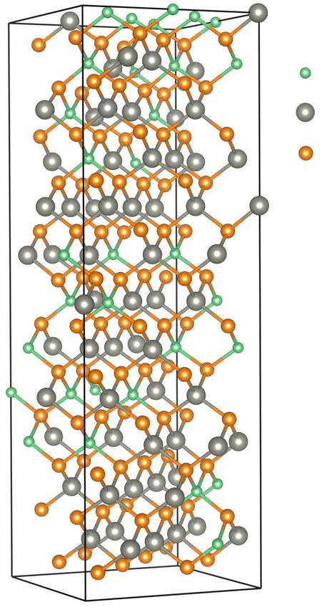
S IESTA                                                                                                                              2

            engaged in the Electronic Structure Library effort from its inception, which has allowed the sharing of various low level
            libraries, as well as data standards and support for them, in particular the PSML definition and library for transferable
            pseudopotentials, and the interface to the ELSI library of solvers. Code sharing is made easier by the new open-source
            licensing model of the program. This review also presents examples of application of the capabilities of the code, as
            well as a view of on-going and future developments.

I.    INTRODUCTION.                                                      As we shall see, the improvements touch many areas. We
                                                                      can underline the implementation of new core electronic-
   The possibility of treating large systems with first-              structure features (DFT+U, spin-orbit interaction, hybrid
principles electronic-structure methods has opened up new re-         functionals), modes of operation (improved time-dependent
search avenues in many disciplines. The S IESTA method and            density functional theory (TD-DFT), density functional per-
its implementation have been key in this development, offer-          turbation theory (DFPT), and analysis methods and proce-
ing an efficient and flexible simulation paradigm based on the        dures to access new properties. A major effort has been spent
use of strictly localized basis sets. This approach enables the       in enhancing the interoperability of the code at various levels
implementation of reduced scaling algorithms, and its accu-           (sharing of pseudopotentials, a new wannierization interface
racy and cost can be tuned in a wide range, from quick ex-            opening the way to sophisticated post-processing, and an in-
ploratory calculations to highly accurate simulations matching        terface to multiscale methods). Very significant performance
the quality of other approaches, such as plane-wave methods.          enhancements have been made, notably to the T RAN S IESTA
   The S IESTA method has been described in detail in Ref. 1,         module through improved algorithms, and to the core elec-
with an update in Ref. 2. In this paper we shall describe its         tronic structure problem through the development of inter-
present status, highlighting its strengths and documenting the        faces to new solvers. These advances have put S IESTA in a
steps that have recently been taken to improve its capabili-          prominent place in the high-performance electronic-structure
ties, performance, ease of use, and visibility in the electronic-     simulation scene, a role reinforced by its participation in im-
structure community.                                                  portant international initiatives and by its new open-source li-
                                                                      censing model.
                                                                         The manuscript is organized as follows. We provide an
                                                                      overview of the underlying methodology and the capabilities
a) Electronic  mail: albertog@icmab.es
b) Electronic
                                                                      of S IESTA in section II, which serves to place the code in the
               mail: nicpa@dtu.dk
c) Electronic mail: arsalan.akhtar@icn2.cat                           wider ecosystem of electronic-structure materials simulation.
d) Electronic mail: ea245@cam.ac.uk                                   Section III presents the recent developments in and around
e) Electronic mail: volker.blum@duke.edu                              the code, which are covered in sub-sections. To showcase
f) Electronic mail: ebosoni@icmab.es                                  S IESTA’s utility in the context of electronic-structure calcula-
g) Electronic mail: pedro_brandimarte001@ehu.eus
                                                                      tions, we present briefly some relevant applications and survey
h) Electronic mail: mabr@dtu.dk
i) Electronic mail: jcerda@icmm.csic.es
                                                                      a few areas in which S IESTA is being profitably used in sec-
j) Electronic mail: fabiano.corsetti@gmail.com                        tion IV. Plans for the future evolution of S IESTA are outlined
k) Electronic mail: ramon.cuadrado@gmail.com                          in section V.
l) Electronic mail: vdikan@icmab.es
m) Electronic mail: ferrer@uniovi.es
n) Electronic mail: J.Gale@curtin.edu.au
o) Electronic mail: garciapa@unican.es                                II.   KEY CONCEPTS OF SIESTA
p) Electronic mail: vm.garciasuarez@gmail.com
q) Electronic mail: sandragil@gmail.com
                                                                      A.    Theory background and context
r) Electronic mail: ghuhs@physik.hu-berlin.de
s) Electronic mail: sergiollera22@gmail.com
t) Electronic mail: korytar@karlov.mff.cuni.cz                           S IESTA appeared as a consequence of the push for linear-
u) Electronic mail: koval.peter@gmail.com                             scaling electronic structure methods of the mid nineties,
v) Electronic mail: i.lebedeva@nanogune.eu
                                                                      which has been reviewed, for example, in Refs. 3 and 4.
w) Electronic mail: linlin@math.berkeley.edu
x) Electronic mail: pablolopeztarifa@gmail.com
                                                                      S IESTA was the first linear-scaling self-consistent implemen-
y) Electronic mail: sara.garciamayo@uam.es                            tation of density functional theory (DFT).5,6
z) Electronic mail: stephan.mohr@bsc.es                                  The S IESTA method relies on atomic-like functions of fi-
aa) Electronic mail: pablo.ordejon@icn2.cat                           nite support as basis sets7,8 – of arbitrary number, angular
bb) Electronic mail: andrei.postnikov@univ-lorraine.fr
                                                                      momentum, radial shape, and centers – combined with a dis-
cc) Electronic mail: yann.pouillon@unican.es
dd) Electronic mail: miguel.pruneda@icn2.cat
                                                                      cretization of space for the computation of the Kohn-Sham
ee) Electronic mail: roberto.robles@ehu.eus                           Hamiltonian terms that involve more than two centers. The
ff) Electronic mail: daniel.sanchez@ehu.eus                           electron-ion interaction is represented by norm-conserving
gg) Electronic mail: jose.soler@uam.es                                pseudopotentials. These key ingredients, through the opti-
hh) Electronic mail: ullah1@llnl.gov                                  mized handling of sparse matrices, are used to compute the
ii) Electronic mail: wenzhe.yu@duke.edu
                                                                      self-consistent Hamiltonian and overlap matrices with a com-
jj) Electronic mail: javier.junquera@unican.es
                                                                      putational expense that scales linearly with system size. The
S IESTA                                                                                                                             3

method is completed with a choice of solvers for that Hamilto-      energies, forces, molecular-dynamics simulations, band struc-
nian, from optimized (but cube-scaling) diagonalization meth-       tures, densities of states, etc., and shares with those codes the
ods, to reduced-scaling solvers of different flavors.               basic current limitations of DFT (notably the description of
   The orbitals in the S IESTA basis set are made of the product    strongly-correlated systems).
of a real spherical harmonic and a radial function, which is nu-       What makes S IESTA different from most other codes, and is
merically tabulated in a grid. The shape of the radial part is in   at the root of its key strengths, is the atomic-like, and strictly
principle totally arbitrary, but the experience accumulated has     localized, character of its basis set. The use of a “good first
proven that the numerical solution of the Schrodinger equa-         approximation” to the full problem implies, first, that a much
tion for a (confined) isolated atom with the corresponding          smaller number of basis functions is needed. Second, the
pseudopotential is a very good choice in terms of accuracy          finite-support of the orbitals leads to sparsity and the possibil-
versus computational cost. Fuller descriptions of the mecha-        ity to use reduced-scaling methods. Thus high performance
nisms to generate and optimize these pseudo-atomic orbitals         emerges almost by default.
(PAOs) are given in Refs. 8–10.                                        Take first the basis cardinality: the number of basis orbital
   The auxiliary real-space grid is an essential ingredient of      per atom in a typical S IESTA calculation is of the order of
the method, as it allows the efficient representation of charge     10-20. This is to be compared with a few hundred in the typ-
densities and potentials, as well as the computation of the ma-     ical plane-wave (PW) calculation. Furthermore, for systems
trix elements of the Hamiltonian that cannot be handled as          whose description needs a vacuum region (e.g., slabs for sur-
two-center integrals. This grid can be seen as the reciprocal       face calculations, 2D monolayers, etc), empty space is essen-
space of a set of plane waves, and its fineness is most conve-      tially “free” for S IESTA, whereas PW codes still need a basis
niently parametrized by an energy cutoff (the “density” cutoff      set determined by the total size of the simulation cell. S IESTA
of plane-wave methods). There are limits to the softness of the     is then quite capable of dealing with systems composed of
functions that can be described with such a grid, so core elec-     dozens to hundreds of atoms on modest hardware, even when
trons are not considered (although semi-core electrons usually      using cubic-scaling diagonalization solvers, which are the de-
are), and their effect is incorporated into pseudopotentials.       fault as they are universally applicable.
The real-space grid is also used to solve the Poisson equation         Electronic-structure solvers with a more favorable size-
involved in the computation of the electrostatic potential from     scaling can be applied to suitable systems. For example, one
the charge density, through the use of a fast-fourier-transform     of S IESTA’s earlier calculations, in 1996, was a linear-scaling
method. This means that S IESTA uses periodic boundary con-         run for a strand of DNA with 650 atoms, performed on a desk-
ditions. Non periodic systems, such as molecules, tubes, or         top workstation of the era.6 Reduced size-scaling is also a
slabs, are treated using appropriate supercells.                    feature of the PEXSI solver described in section III G 1 be-
   S IESTA is now a mature code with more than 20 years of          low, and of the NTPoly solver mentioned in section III G 2.
existence. In this period, the most important algorithms be-        In addition to time-to-solution efficiency, these solvers have
hind our implementation have been already fully described           a smaller memory footprint than diagonalization, as the rele-
and documented in a series of papers. Readers interested in         vant matrices are kept in sparse form rather than converted to
the details of how the basic elements defining the method are       a dense format.
combined, as well as other relevant implementation details             Crucially, S IESTA’s baseline efficiency can be scaled up to
that make the method practical, can find them in the main           ever-larger systems by parallelization. Both distributed (MPI)
S IESTA reference1 , and in the update with the new capabil-        and shared-memory (OpenMP) parallelization options are im-
ities of the code2 .                                                plemented in the code. As some of the examples in section IV
   We note that the term S IESTA is regularly used to describe      show, non-trivial calculations with thousands of atoms are
both the method (as outlined in the earliest papers5,6 ) and its    used in applications in different contexts, from molecular bi-
implementation in a computer program. The S IESTA method            ology to electronic transport.
is at the basis of later independent implementations, such             Work on the performance aspects of the code is continu-
as OpenMX,11 and QuantumATK.12 Other subsequent codes               ous, mostly on the solvers, which usually take most of the
built on the method, revising some of the fundamental ingre-        computer time due to the very high efficiency of the Hamilto-
dients. This is the case of FHI-aims,13 which uses a more           nian setup module in S IESTA. This task is facilitated (see sec-
sophisticated real-space grid (atom-centered), thus extending       tion III O) by leveraging external libraries and developments
the core scheme to all-electron calculations.                       generated by a number of international initiatives in which
   In this paper we describe new additions to the S IESTA code,     S IESTA participates. The code can still run efficiently in mod-
based on independent methodological advances, either pre-           est hardware, while also being able to exploit massive levels
existent or specifically developed for S IESTA, as specified and    of parallelism in large supercomputers (see Fig. 1).
cited in each section below.                                           It is worth noting also that the atomic character of the basis
                                                                    set enables the use of a very intuitive suite of analysis tools,
                                                                    sice most of the concepts relating to chemical bonding use the
B.   Overview of Siesta capabilities                                language of atomic orbitals. Hence S IESTA has a natural ad-
                                                                    vantage in this area. Partial densities of states and atomic and
   As a general purpose implementation, S IESTA can provide         crystal populations (COOP/COHP) are routinely used to gain
the standard functionality available in mainstream DFT codes:       insights into the stability and other properties of materials.
for ScaLAPACK, Siesta-PEXSI needs only 144 cores for
C-BN0.00 and 64 for DNA-25. In the case of DNA even
this minimal configuration is more than four times faster
proach Sthan
IESTAdiagonalization with 5120 processors. 4
Strong scaling
the base the community, shared by some of the most popular electronic
cost with structure codes.
ase of the Fourth, with regard to S IESTA specific approximations, par-
trong scal- ticularly the basis set, it should be stressed that S IESTA is lim-
alculating ited to basis sets composed of functions that are product of a
Hamilto- 180,000 orbs radial part and spherical harmonics, but it does not constrain
ion of the 170,000 orbs
2D, sp=0.91%
on how many, where such functions are centered, and the size
aLAPACK 1D, sp=0.27%
of their finite-support region. Calculations can flexibly range
h requires from quick exploration to very high-quality simulations (one
ration. In may recall that accuracy gold standards in electronic struc-
the chem-
ture are provided by quantum-chemistry methods, based on
number of
, reducing
LCAO).
The use of an atomic-orbital basis set implies however the
gh perfor- limitation of non-uniformity of convergence. As opposed to
allelization plane-wave methods, in which a single energy cutoff param-
ntly. The FIG.1.2. Parallel
FIG. Strong strong
scalingscaling
of C-BNof 0.00 and DNA-25
SIESTA-PEXSI andbased on
the (Scala- eter monotonically determines the quality of the calculation,
uning the the total
pack) time for the
diagonalization first SCF
approach for step.
a DNAThe various
chain and alines for
Graphene- there is no univocal procedure for the choice of an appropri-
number of PEXSINitride
Boron result stack,
from using di↵erent
prototypes numbers
of large of processors
(hundreds per of
of thousands ate basis set. It is a well-known problem, shared by the whole
pole (ppp),
orbitals) quasiwhile the points on
one-dimensional andeach curve belongsystems.
two-dimensional to compu- “ppp”
is demon- quantum-chemistry community, on which there is widely used
tationsforwith
stands 1, 2, 5, 10,
the number 20, and
of MPI 40 poles
processes usedininparallel.
each pole computa-
C-BN sys- and tested know-how. As Fig. 2 shows, it is possible to attain
me ppp are tion, and “sp” the sparsity of the Hamiltonian. (For more details, see in practice an accuracy comparable to that of well-converged
ling. The PEXSI’s
section III G 1)beneficial scaling with the system size, as de- plane-wave calculations. The reader is also referred to sec-
ation over scribed in section II C, guarantees that for large enough tions IV B and IV C 1 for showcase examples of the accuracy
paralleliza- systems Siesta-PEXSI will always be faster than diag-
of the code, among many others in the literature.
come from onalization. The scaling of the computational cost is
For a recent example,
demonstrated for DNA seeand
Ref.C-BN
14. Similarly,
in figure 3. an atomic basis To close this section, we stress that it has been a tradi-
only a lim- tional and deliberate attitude by the S IESTA team that, al-
thus does provides
In all tests full parallelization over poles is for
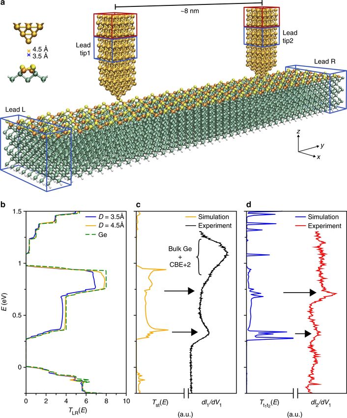
a very natural and adequate language the In
used. first-
principles simulation of electronic ballistic
this configuration the influence of the symbolic factoriza- transport in nano- though proposing sensible starting points to users as defaults,
able. This
currently sized systems,
tion would via the
change the Green’s-function
character of the method. based Keldysh
Becausefor- the choice of fundamental approximations and inputs to the
e time for malism
in futureimplemented
this influence in T RAN
will SbeIESTA ,15 a partthe
negligible, of time
the S IESTA
for program (not only basis sets, but also density functionals, and
nal role. package.
symbolic factorization is not taken into account for the pseudopotentials) is a responsibility of the users, who retain
e, demon- analysis. full control and the flexibility to adapt the code to their specific
The very high number of citations of the S IESTA papers
Thetonumbers of processes for each needs. Nevertheless, tools for basis optimization are provided
es treated testify the successful application of system
the codesize are cho-dif-
to widely
sen to be an efficient trade-o↵ of reducing the time with the program, new curated databases of pseudopotentials
rther, but ferent systems. With regard to specific capabilities andtothe
on. [LL: solution while keeping the cost, which increases with the are coming online, and new ways to ameliorate the correlation
levels of accuracy achievable, we can distinguish several lev-
the scaling number of processes due to inefficiencies, as small as pos- problem are being implemented. Some of these developments
els. First, S IESTA implements DFT, one of the most versatile
time by a sible. Following this guideline it turns out, that for C- are described in the following sections.
materials
BN one can simulation
use moreframeworks.
processors with DFTSiesta-PEXSI
has its shortcomings,
than
both ex- notably
with ScaLAPACK. This also means, that the advantagesys-
in regard to the description of strongly-correlated
hroughout tems, but these areinbeing
of Siesta-PEXSI termsaddressed (see sections
of solution-time is even onlarger
DFT+U
III. RECENT DEVELOPMENTS IN SIESTA
of Siesta- and
thanhybrid functionals
the benefit of cost.below).
For verySecond,
sparseS IESTA
problems, useslike
pseu-
PEXSI ap- dopotentials
the largest DNA examples, the amount of processors thatThe
to represent the electron-ion interaction.
pseudopotential
can be used is approach similar for is firmly rooted in abut
both methods, sound physi-
Siesta- A. New distribution model and development infrastructure
allows an
the scalig cal approximation
PEXSI is about two (thatorders
bonding of effects
magnitude depend mostly
faster. on the
More
this. For details electrons);
valence are listed inhowever,
table II.it is at a disadvantage when core- A few years ago, in 2016, a decision was made to change
ce this ex- The analysis
electrons effects areshows, besides(but
important Siesta-PEXSI’s
see section IIIfavorable
N 6 below). the licensing model for S IESTA: traditionally it had always
Third, S IESTA employs periodic boundary conditions (PBC) been free of charge to academics, but non-academic use re-
for the solution of the Poisson problem, sharing with plane- quired a special license and redistribution was not permitted.
wave codes the need to resort to repeated supercells for the Now S IESTA is formally an open-source program, distributed
study of low-dimensional systems, and to special techniques according to the terms of the GPL license18 . At the same
for the treatment of charged systems. It is important to note, time, the development infrastructure was made more trans-
however, that, unlike plane-wave codes, S IESTA is only bound parent and scalable, using first the Launchpad platform19 and
to PBC because of the present treatment of the Hartree term now the Gitlab service20 . The net effect of the changes has
of the single-particle Hamiltonian. This limitation is lifted by been a more fertile and dynamic development, with more con-
the incorporation of alternative Poisson solvers, as described tributors who can have direct access to the various branches
in Sec. III O, which allow for open boundary conditions, as of development, and a better experience for users, who can
for isolated nano-systems, and hybrid open/periodic bound- download code and raise issues in an integrated platform.
ary conditions in different dimensions, as for isolated wires These changes have been substantial for the core develop-
and slabs. It should be remembered that the three approxi- ers, and the transitory period is still being felt. The main code
mations mentioned in this paragraph are very widely used in base is gradually absorbing new developments, both those that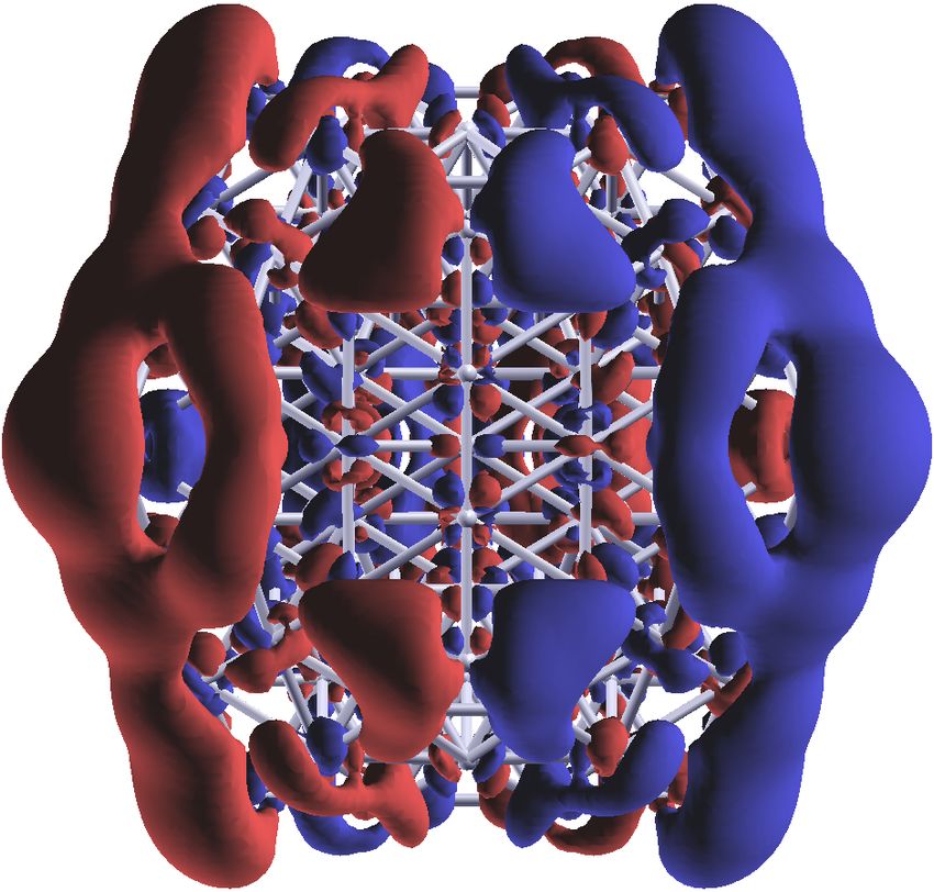
S IESTA                                                                                                                                               5

                                                                                     norm-conserving pseudopotentials, easing in most cases the
                                        0.0
                                                                                     task of pseudopotential quality control.
            250

                              (meV)
                                        -0.4

                             PW
                                                                                     C.   DFT+U for correlated systems

                              Eb - Eb
 Eb (meV)

                                        -0.8
            240
                                                                                        The LDA+U method, initially developed by Anisimov and
                                               70     75        80     85       90
                                                                                     coworkers28 with the objective to improve the treatment of the
                                                    Number of basis functions
                                                                                     electron-electron interaction for localized electrons within the
                                                                                     bare LDA description, has been implemented in S IESTA. The
            230   PW
                                                                                     idea behind the LDA+U consists in describing the “strongly
                                                                                     correlated” electronic states of a system (typically, localized
                       30               50                 70                   90   d or f orbitals) using the Hubbard model, whereas the rest of
                             Number of basis functions                               valence electrons are treated at the level of “standard” approx-
                                                                                     imate DFT functionals.29 In the current version of S IESTA the
FIG. 2. Basis set convergence for the binding energy (Eb ) of a water                implementation is based on the simplified rotationally invari-
dimer. Details can be found in Ref. 16. The horizontal dotted line                   ant functional proposed by Dudarev and coworkers.30 Here,
represents the converged plane-wave (PW) calculation (1300 eV cut-                   the corrections are made invariant under rotation of the atomic
off) for the same system (dimer geometry and box), pseudopotentials                  orbitals used to define the occupation number of the correlated
and density functional, using the ABINIT code.17 Inset: deviation of                 subspace, at the cost of retaining only the lowest order Slater
Eb versus the PW reference. The deviation for the last point is of 10                integrals in the factorization of the integrals of the Coulomb
µeV.
                                                                                     kernel of the electron-electron interaction, and neglecting the
                                                                                     higher order ones (i.e. taking the exchange interaction J as 0).
                                                                                     The expression of the corrective term as a functional of the
were planned long in advance, and new ones made possible by                          occupation number nIσ  `m of the localized correlated orbital `m
the greater openness and fluidity of the development model.                          with spin σ within the atom I is given by
Most of the new features described below are already part of
public releases, but a few are undergoing the last stages of
                                                                                                             U I`

testing before release. The work-flow is also moving from                                           EU = ∑                  nIσ   1 − nIσ

                                                                                                                                                 ,   (1)
                                                                                                                    ∑        `m        `m
long-lived releases, hard to maintain with bug-fixes, to more                                            Iσ ` 2         m
frequent releases that will be maintained for a shorter time.
                                                                                     where only one interaction parameter U I` is needed to specify
                                                                                     the interaction per atom and `-shell. In the practical S IESTA
                                                                                     implementation, the populations on the correlated orbitals are
B.          New pseudopotential format for interoperability
                                                                                     computed using non-overlapping (i. e. orthogonal) localized
                                                                                     projectors. They can be generated using either (i) the same
   PSML (for PSeudopotential Markup Language)21,22 is a file                         algorithm used to produce the first-ζ orbitals of the basis set,
format for norm-conserving pseudopotential data which is de-                         but with a larger energy shift, or (ii) cutting the exact solution
signed to encapsulate as much as possible the abstract con-                          of the pseudoatom with a Fermi function.
cepts involved in the domain, and to provide appropriate meta-                          The results of the LDA+U method are sensitively depen-
data and provenance information. This extra level of formal-                         dent on the numerical value of the effective on-site electronic
ization aims at removing the interoperability problems associ-                       interaction, the Hubbard U. Although in principle the value
ated to bespoke pseudopotential formats, which usually were                          of U can be computed from first principles using linear re-
designed to serve the needs of specific generators and client                        sponse methods,31 a common practice is to tune it semiempir-
codes, and thus contain implicit assumptions about the mean-                         ically, seeking agreement of certain properties (for instance
ing of the data or lack information not considered relevant.                         band gaps or magnetic moments) with available experimen-
   PSML files can be produced by the ONCVPSP23 and                                   tal measurements. Then, the fitted U is used in subsequent
ATOM24 pseudopotential generator programs, and are a                                 calculations to predict other properties.
download-format option in the Pseudo-Dojo database of cu-                               The LDA+U corrects localized states, for which the self-
rated pseudopotentials25,26 .                                                        interaction correction is expected to be stronger, and is an ef-
   The software library libPSML21,22 can be used by elec-                            fective method to improve the description of the (underesti-
tronic structure codes to transparently extract the information                      mated) band gap of insulators, as shown in Fig. 3 for the case
in a PSML file and incorporate it into their own data struc-                         of NiO. Once the Hubbard correction is switched on, the op-
tures, or to create converters for other formats. It is cur-                         tical band gap increases up to 3.08 eV (from the bare GGA-
rently used by S IESTA and A BINIT,17,27 making possible a                           PBE value of 1.08 eV), very close to the experimental value
full pseudopotential interoperability and facilitating compar-                       for the onset of optical absorption in NiO32 (3.10 eV). The
isons of calculation results.                                                        magnetic moment on the Ni atom is also properly described,
   The use of this new format opens the door to benefit from                         with a value of 1.67 µB which lies well within the experi-
the availability of a periodic table of reliable and accurate                        mental range of values (between 1.64 µB 33 and 1.9 µB 34 ), and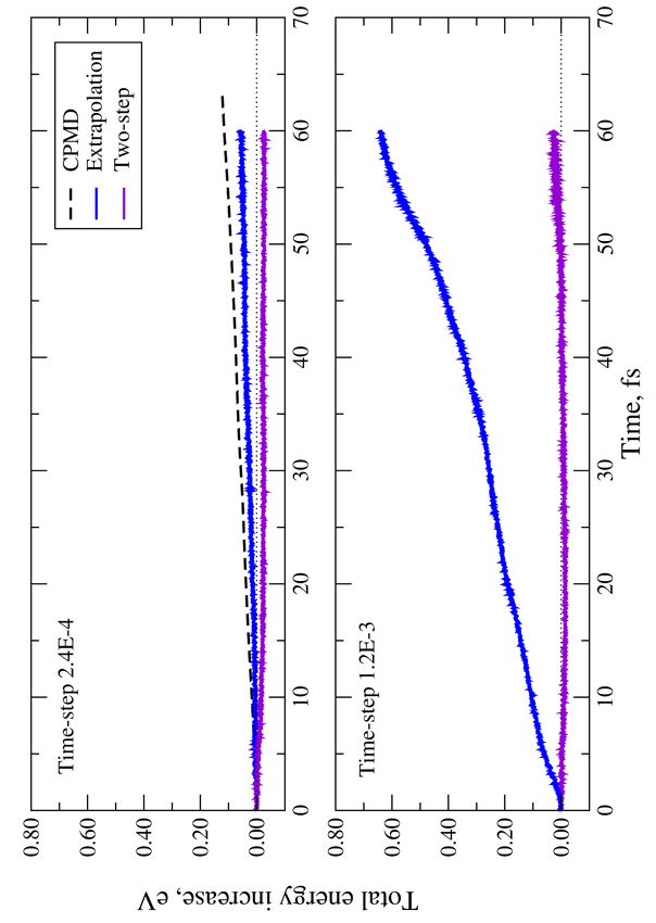
S IESTA                                                                                                                                 6

improves on the result of 1.39 µB obtained with a bare GGA-              E.   Hybrid functionals
PBE functional.
                                                                            The screened hybrid functional HSE0642–44 has been im-
                         5                                               plemented in S IESTA building on the work of Ref. 45. This
                                                                         functional is the result of adding nonlocal Hartree-Fock type
                                                                         exact exchange (HFX) into semilocal density functionals. The
                                                                         Coulomb potential that appears in the exchange interaction is
                         0                                               screened, so it has a shorter range than 1/r. Here, to reduce
                                                                         the big prefactor involved in the computation of the HFX po-
          Energy (eV)

                                                                         tential matrix elements, we fit the NAO of the basis set with
                                                                         Gaussian-type orbitals, specially suited to computing the four
                                                                         center electron repulsion integrals (ERIs) in a straightforward
                         -5
                                                                         and efficient analytical way. An example of this fitting for the
                                                                         2s and 2p atomic orbitals basis set of the oxygen is shown
                                                                         in Fig. 4. The LIBINT package46 is required to calculate
                                                      (a)                primitive ERIs, where recursive schemes of the Obara-Saika47
                        -10
                           Γ   L   K    T     Γ             X            method and the Head-Gordon and Pople’s variation48 thereof
                          5                                              are implemented. ERIs are calculated in the first SCF cycle
                                                                         and then stored in disk. Only the ERIs with non-negligible
                                                                         contributions are calculated, keeping the HFX Hamiltonian
                                                                         also sparse.
                         0                                                  This HSE06 functional has been used to compute the band
          Energy (eV)

                                                                         structure of bulk Si [diamond structure; Fig. 5(a)] and BaTiO3
                                                                         [cubic structure; Fig. 5(b)] with a double-zeta polarized basis
                                                                         set at the equilibrium lattice constant of the Perdew-Burke-
                         -5                                              Ernzerhof functional49 within the Generalized Gradient Ap-
                                                                         proximation (5.499 Å for Si and 4.033 Å for BaTiO3 ). In
                                                                         both cases, the gap is opened with respect to the value ob-
                                                      (b)
                                                                         tained with the semilocal functional. In bulk Si the band gap
                        -10
                                                                         is indirect: the top of the valence band is located at Γ and the
                           Γ   L   K    T     Γ             X            bottom of the conduction band at a point along the Γ → X
                                                                         high-symmetry line. It increases from 0.64 eV within GGA
FIG. 3. Band structure of NiO in the undistorted rock-salt type struc-   to 1.00 eV with the hybrid functional, in good agreement with
ture with rhombohedral symmetry introduced by a type-II antiferro-
                                                                         the experimental value of 1.17 eV50 . For the case of the per-
magnetic order. The experimental lattice spacing is used. The bands
obtained within GGA-Perdew-Burke-Ernzerhof functional (panel a),         ovskite oxide BaTiO3 , the band gap is also indirect, from R to
and with a Hubbard U correction of 4.6 eV applied on the d-orbitals      Γ, and its value increases from 1.87 eV with GGA to 3.28 eV
of Ni (panel b), as in Ref. 31, are shown. The zero of the energy is     with the HSE06 functional, almost matching the experimental
set at the top of the valence band.                                      value of 3.2 eV estimated by Wemple in the cubic phase51 .

                                                                         F.   Spin-orbit coupling

                                                                            The capability to include the spin–orbit (SO) interaction in
D.   Van der Waals functionals
                                                                         S IESTA and in the analysis tools is seen as a strategic asset
                                                                         for the project in view of the recent interest in topological in-
   An efficient calculation of van der Waals (vdW)                       sulators and quasi–two–dimensional systems with important
functionals35,36 was developed and first implemented in                  spin–orbit effects, like some of the transition metal dichalco-
S IESTA using a polynomial expansion in the local variables              genides. Also, it brings the possibility to obtain the magnetic
(q1 , q2 ) of the nonlocal interaction kernel Φ(q1 , q2 , r12 ) and a    crystalline anisotropy (MCA) (change in the total energy of
Fourier expansion in the relative position r12 37 . As a result,         the system upon changing the spin quantization axis).
the scaling of the vdW computation decreases from O(N 2 ) to                In a standard collinear-spin DFT calculation, the total KS
O(N log N) and it becomes marginal within the overall cost.              Hamiltonian is represented by two independent spin–blocks,
This scheme was later extended16 to a more complex kernel38                 σ σ [σ =↑, ↓]. However, when the SO coupling is included,
                                                                         Ĥµν
of the form Φ(n1 , |∇n1 |, n2 , |∇n2 |, r12 ), and it has been applied   off–diagonal spin blocks arise (i.e., there are non–zero cou-
to a large variety of systems, like carbon nanotubes37 , hydro-          plings between the two spin components). Therefore, and
gen adsorption39,40 , or liquid water41 .                                similar to the non-collinear spin case, the Hamiltonian be-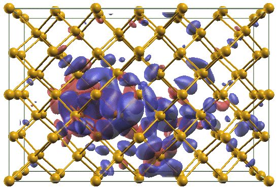
S IESTA                                                                                                                                        7

                                                                                            10
          1.4

          1.2

          1.0                                                                                5
          0.8
    Rnl (r)
     rl

                                                                              Energy (eV)
          0.6                                                                                0
          0.4

          0.2
                                                                                             -5
          0.0     0.5         1.0         1.5         2.0     2.5
                                           r (Bohr)

                                                                                            -10
          5.0
                                                                                                                                     (a)
          4.0                                                                               -15
                                                                                               L       Γ        X       W K                Γ
                                                                                             8
    Rnl (r)

          3.0
     rl

          2.0
                                                                                            6
          1.0

                                                                                            4
          0.0    0.5    1.0         1.5         2.0     2.5
                                           r (Bohr)                           Energy (eV)
                                                                                            2
FIG. 4. Gaussian fits of the radial part of oxygen 2s (a) and 2p (b) or-
bitals using 6 Gaussian functions. The orbitals to fit are represented
                                                                                            0
by blue dots and the corresponding Gaussian expansions by green
continuous lines. Dashed vertical lines represent the standard devi-
ations of individual Gaussians and a red continuous line marks their                        -2
upper limit. The orbitals are set to zero in the yellow area, marking
their cutoff radii.
                                                                                            -4
                                                                                                                                     (b)
comes a full 2×2 matrix in spin space                                                       -6
                                                                                              Γ    X   M   R        Γ      M     X         R
                                                  ↑↑   ↑↓
                                                              !
                          KS                    Ĥµν Ĥµν
                        Ĥµν =                    ↓↑   ↓↓
                                                                    (2)    FIG. 5. Band structure of (a) bulk Si in the diamond structure, and
                                                Ĥµν Ĥµν                  (b) bulk BaTiO3 in the cubic structure obtained with the Perdew-
                                                                           Burke-Ernzerhof functional (red lines) and with the HSE06 hybrid
where µν subindexes refer to the S IESTA basis orbitals. The               functional (black lines). The zero of energies have been set to the
fully relativistic Hamiltonian Ĥ KS is expressed as a sum of the          valence band maximum.
kinetic energy T̂ , the scalar-relativistic pseudo-potential part
in the form of Kleinman–Bylander projectors V̂ KB , the spin–
orbit V̂ SO term and the Hartree V̂ H and exchange–correlation                In the current implementation the SO term is included
V̂ XC potentials:                                                          non-perturbatively, so that the fully relativistic Hamiltonian
                                                                           is solved self-consistently after extending the Kohn–Sham
                Ĥ KS = T̂ + V̂ KB + V̂ SO + V̂ H + V̂ XC           (3)    wave–functions to full spinors. Two different approaches have
                                                                           been implemented in S IESTA to account for the SO term, V̂ SO :
The first three terms of the right hand side do not depend on                      - on–site approximation:
the charge density, ρ(r), and therefore do not change in the                         Based on the work of Fernández-Seivane et al. 53,54 ,
self–consistent cycle, while V̂ SO and V̂ XC are the only spin–                      only the intra–atomic SO contributions within each l–
dependent terms that couple both spin components.                                    shell of each atom are considered. In this approach the
   In order to compute the MCAs, different orientations of                           SO terms are obtained from analytical simple expres-
the spin quantization axis need to be considered. This may                           sions for the angular integrals while the radial integrals
be done by rotating either V̂ SO (as done by Cuadrado and                            are computed numerically.
Cerdá 52 ) or the density matrix, which is the approach cur-
rently followed by S IESTA for compatibility with the non–                         - off–site approach:
collinear case.                                                                      Here, V̂ SO is built        following     the   Hemstreet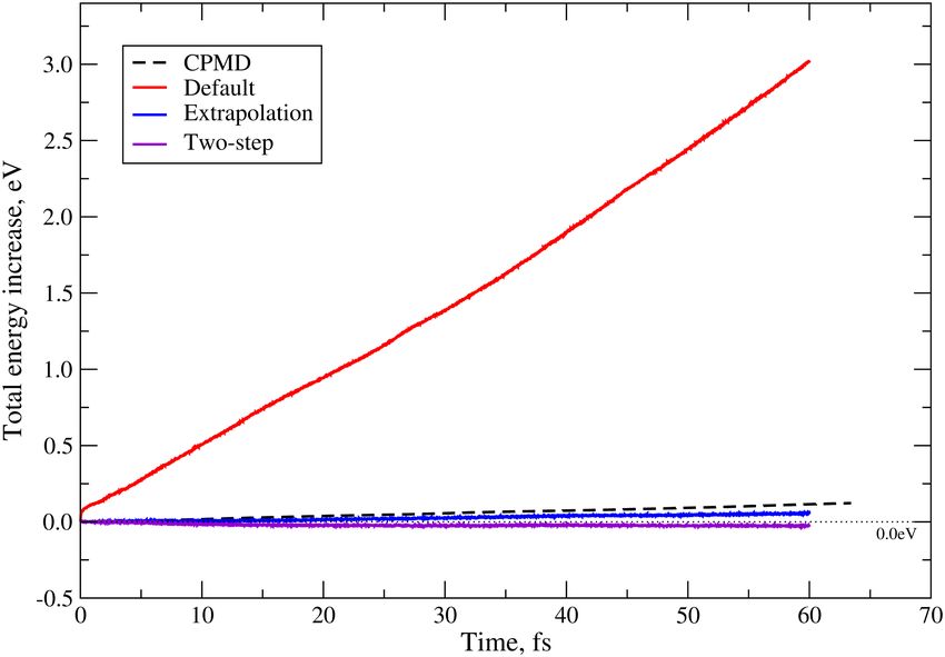
S IESTA                                                                                                                           8

      formalism52,55 whereby a fully-relativistic pseudo-               • The Fermi Operator Expansion method (FOE)63 uses
      potential (FR-PP) operator is constructed in a fully                the formal relationship between Hamiltonian and
      separable form, i.e., non–local in the radial part                  density-matrix, ρ̂ = fFD (Ĥ − µ), where fFD is the
      as well as in the angular variables, in order to                    Fermi-Dirac function. A simple polynomial expansion
      substantially reduce the computational cost. The                    of fFD can then be used to obtain ρ̂ without diagonal-
      necessary l j Kleinman–Bylander projectors may be                   ization. This method is implemented in the CheSS li-
      either constructed by S IESTA itself from relativistic              brary64 , developed within the BigDFT project65 .
      semilocal PPs, or directly read from appropriately
      generated PSML files, as provided by the Pseudo–                  • The PEXSI method66,67 uses a pole expansion of fFD to
      Dojo project25,26 . Moreover, we note that the FR-PP                get ρ̂ in the form:
      formalism (as well as the original one implemented
      in Ref. 52) uses the correct normalization constants                                                         !
                                                                                                P        ρ
      Cl±1/2 , in contrast with what was erroneously stated in                                          ωl
                                                                                       ρ̂ = Im ∑                                (4)
      Ref. 56.
                                                                                               l=1 H − (zl + µ)S
   Although we consider the off–site approach more accurate,
                                                                                   ρ
as it includes inter-shell and inter-atomic SO couplings, both            where ωl and zl are the weights and poles for the cor-
approximations yield very similar results in most of the tested           responding expansion of the Fermi-Dirac function. The
systems, with relevant qualitative differences only found in a            number of poles needed is significantly smaller than for
few specific cases. Furthermore, the construction of the Vµν SO           the polynomial version of the FOE, as its dependence
matrix is very fast under both schemes and involves a tiny                on the spectrum size is only logarithmic.
fraction of the entire self-consistent calculation.                       It would appear that having to invert matrices would
                                                                          still render this approach cubic-scaling, but in fact
                                                                          only selected elements of ρ̂ have to be actually com-
G.   New electronic-structure solvers
                                                                          puted. This “pole expansion and selected inversion”
                                                                          method offers a reduced complexity (at most O(N 2 )
   For most problems, S IESTA spends the largest fraction of              for dense systems, and O(N) for quasi-one-dimensional
cpu-time in the solver stage (solution of the generalized eigen-          systems), and trivial parallelization over poles, so it is
value problem HΦ = εSΦ). The stage devoted to the calcu-                  well-suited for very large problems on large machines.
lation of the hamiltonian H and overlap S is typically much               For example,68 computed the electronic structure of
lighter weight, as those matrices are intrinsically sparse due            large (up to 11,700 atoms) graphene nanoflakes using
to the use of a finite-support basis set. Accordingly, S IESTA’s          S IESTA-PEXSI.
performance is almost completely linked to the use of appro-
priate external solver libraries.                                       • The electronic structure problem can also be cast as a
   Over the past few years we have expanded the choices avail-            minimization problem (of an extended functional) with-
able to users and refined the relevant interfaces. Initially, we          out orthogonalization. When additional localization
added support for new individual solvers as detailed below,               constraints are put in place, the original linear-scaling
but recently we have consolidated some of the most impor-                 method in S IESTA results. Without the extra localiza-
tant functionality under a new common interface to the ELSI               tion constraints, the cubic-scaling Orbital Minimization
library of solvers57,58 .                                                 Method (OMM)69 can be competitive with respect to
                                                                          diagonalization, as data can be reused across scf-cycle
                                                                          steps.
1.   Solvers with a native interface

   Diagonalization (solution of the generalized eigenproblem       2.   The ELSI interface
appropriate for non-orthogonal orbitals) is the default method
for obtaining the density-matrix in S IESTA. A number of stan-        We have considerably extended the range of solver choices
dard routines are contained in the S CA LAPACK library59 ,         and the performance enhancement possibilities of the code
but more efficient alternatives are possible. In particular, the   with the integration of the open-source ELSI library (https:
ELPA library60–62 uses an extra intermediate step in the tridi-    //elsi-interchange.org), that provides a unified soft-
agonal conversion of the matrices to obtain better scalability     ware interface that connects electronic structure codes to var-
and significant speedups over S CA LAPACK. An interface to         ious high-performance solver libraries to solve or circumvent
ELPA is offered in S IESTA, so this solver can be used as a        eigenproblems encountered in electronic structure theory57 .
drop-in replacement for S CA LAPACK throughout the code.           ELSI also ships with its own tested versions of the individual
   In addition, S IESTA has implemented interfaces to several      solver libraries, but additionally, linking against already com-
methods not based on diagonalization. In most cases, the           piled upstream versions from each solver library is supported
use of a finite-support basis set, leading to the appearance of    as much as possible.
sparse matrices, is a significant factor to achieve good perfor-      The ELPA, OMM, and PEXSI solvers, which had their
mance:                                                             own ad-hoc interfaces as described in the previous section,
S IESTA                                                                                                                                                     9

are now available through ELSI, which also supports other                                  over trial points for the determination of the chemical-
conventional dense eigensolvers (EigenExa70 , MAGMA71 ),                                   potential.
sparse iterative eigensolvers (SLEPc72 ), and linear scaling
density matrix purification methods (NTPoly73 ). As sketched                             • Mixed-precision support: The ELPA solver can be in-
in Fig. 6, an electronic structure code interfacing to ELSI au-                            voked in single-precision mode, which can speed up the
tomatically has access to all the eigensolvers and density ma-                             initial steps of the electronic self-consistent-field (scf)
trix solvers supported in ELSI. In addition, the ELSI inter-                               cycle.
face is able to convert arbitrarily distributed dense and sparse                         • Accelerator offloading: The ELPA library offers GPU
matrices to the specification expected by the solvers, taking                              support in some kernels62 , and there is scope for ex-
this burden away from the electronic structure code. A com-                                tending it to more kernels. ELSI also offers an interface
prehensive review of the capabilities in the latest version of                             to the accelerator-enabled MAGMA library. Finally, the
ELSI, including parallel solution of problems found in spin-                               PEXSI developers are working on adding GPU support
polarized systems (two spin channels) and periodic systems                                 to the solver.
(multiple k-points), scalable matrix I/O, density matrix ex-
trapolation, iterative eigensolvers in a reverse communication
                                                                                          1024
interface (RCI) framework, has recently been completed58 .                                                                              Scalapack
                                                                                                                                      Siesta-ELPA
                                                                                                                           ELSI-ELPA multi-k-point
                                                                                           512                                               Ideal

                                                                          CPU time (s)
                                                                                           256

                                                                                           128

                                                                                            64

                                                                                            32
                                                                                                 64       128          256            512            1024
                                                                                                                    MPI ranks

                                                                         FIG. 7. Performance improvement from the use of the extra level of
                                                                         parallelization over k-points in S IESTA using the ELSI interface with
                                                                         the ELPA solver, compared to the previous diagonalization scheme
                                                                         (using both the standard S CA LAPACK solver and the existing ELPA
                                                                         interface in S IESTA). The system is bulk Si with H impurities, with
                                                                         1040 atoms, 13328 orbitals, and a sampling of 8 k-points. The multi-
                                                                         k scheme is able to stay closer to ideal scalability for larger numbers
                                                                         of MPI processes.
FIG. 6. Interaction of the ELSI interface with electronic structure
codes. ELSI serves as a bridge between electronic structure codes
and solver libraries. An electronic structure code has access to vari-
ous eigensolvers and density matrix solvers via the ELSI API. When-      H.              Time dependent DFT
ever necessary, ELSI handles the conversion between different units,
conventions, matrix formats, and programming languages.
                                                                            Time-dependent density-functional theory (TD-DFT) was
                                                                         first implemented into S IESTA in its real-time propagating
  With the common interface in place, any additions and en-              form. It was first described in Ref. 74, and then briefly in
hancements to the supported solvers can be used in S IESTA               Ref. 2. It was based on the Crank-Nicolson algorithm, by
with almost no code changes. This is particularly relevant for           which, the effect of the evolution operator for an infinitesimal
performance enhancements. For example:                                   time step
    • Further levels of parallelization: A feature common in

                                                                                        Û(t0 + ∆t,t0 ) = exp −iĤ(t)∆t               (5)
      principle to all solvers is that the S IESTA-ELSI inter-
      face can exploit the full parallelization over k-points            on the wave-function coefficients matrix at a given time t0 ,
      and spins mentioned above. This means that these cal-              c(t0 ) is approximated by
      culations can use two extra levels of parallelization in
                                                                                                         ∆t −1

      the solver step beyond the standard one of paralleliza-                                                                ∆t
                                                                           c(t0 + ∆t) = S + iH(t0 + ∆t)          S − iH(t0 )      c(t0 )
      tion over orbitals (see Fig. 7).                                                                    2                  2
                                                                                                                                       (6)
    • The new version of the PEXSI solver integrated in                  where ∆t represents the finite time-step resulting from time
      ELSI can achieve the same level of precision with                  discretization, and S and H represent the overlap and Hamil-
      fewer poles, and offers an extra level of parallelization          tonian matrices, respectively, in the representation given by
S IESTA                                                                                                                              10

a non-orthogonal basis set, as used by S IESTA. That expres-         steps per atomic motion step, if the nuclei are still significantly
sion is obtained from equating the first-order evolution of the      slower than electrons, for instance. The implementation of the
coefficients forward, from t0 to t0 +∆t/2, to the backward evo-      Crank-Nicolson part is the same for both the fixed and moving
lution from t0 + ∆t to the same intermediate step.                   basis.
   It can be further simplified to                                      The square root and inverse square root are calculated by
                                                                     first computing its eigenvalues and eigenvectors,
                            ∆t −1

                                              ∆t
   c(t0 + ∆t) = S + iH(t0 )       S − iH(t0 )      c(t0 )      (7)                             S = U E U †,                        (12)
                            2                 2

for a smooth-enough variation of the Hamiltonian itself and          where E is a diagonal matrix with the eigenvalues of S. And
a small enough ∆t, thereby avoiding the self-consistency im-         U is a square matrix with the eigenvectors of S as its columns.
plied in propagation using Eq. 6. In Section III H 3 below,          Then,
recent developments on efficient treatments of Eq. 6 beyond
Eq. 7 are presented. Here we describe the parallelization and                S1/2 = U E 1/2U † ,   and    S−1/2 = U E −1/2U †
related features in the TD-DFT implementation now found in
                                                                     where E 1/2 and E −1/2 are obtained by replacing diagonal el-
standard S IESTA releases.
                                                                     ements of E with their square root and inverse square root
   The implemented propagation is based on Eq. (7) (with the         (in the latter case neglecting those eigenvalues below certain
improvement possibilities described in Section III H 3), but         threshold value), respectively.
proper consideration must be taken of the fact that not only            The two-stage algorithm has been implemented in S IESTA
the coefficients change in time, but also the basis set and the      in parallel, allowing for k-point sampling and for collinear
Hilbert space spanned by it when the atoms move. An analy-           spin. The initial occupied states to be propagated are read
sis of the geometrical implications of this fact is presented in     from a file. S IESTA is prepared to run a conventional DFT
Ref. 75. The time-dependent Kohn-Sham equation                       calculation of whatever relevant initial state, and write a wave-
                                                                     function continuation file that acts as initialization of the ul-
                         H|ψi = i∂t |ψi                        (8)
                                                                     terior S IESTA run in real-time TD-DFT mode. As it stands,
becomes                                                              S IESTA evolves states defined as fully occupied; partial occu-
                                                                     pations are not currently supported.
                        Hc = i S (∂t + D)c                     (9)

where H, S, and c are the Hamiltonian, overlap and coeffi-           1.   Parallelization
cients matrices, respectively, as before, and the D matrix is
the connection in the manifold given by the evolving Hilbert            The two-step procedure described above requires matrix-
space75 , Dµν = hφµ |∂t φν i, for φµ and φν basis functions.         matrix and matrix-scalar multiplication, matrix addition, and
   A way of taking such evolution into account in the                matrix inversion, plus the diagonalization of the overlap ma-
discretized implementation was proposed by Tomfohr and               trix for the Löwdin step. Since only the occupied states are
Sankey76 , and is based on a Löwdin orthonormalization. The          propagated, the c matrix is rectangular N × N , that is, num-
scheme consists of two steps. First the wavefunctions are            ber of propagating states × number of basis functions, while
propagated using both S and H at time t0 using Eq. (7), but          S and H are square, N × N . The computation of the overlap
to an auxiliary coefficient matrix c̃,                               and Hamiltonian matrices is handled by pre-existing S IESTA
                                                                     routines, which are already parallelized and well-optimized
                            ∆t −1                                    for HPC environments69,81 .

                                              ∆t
  c̃(t0 + ∆t) = S + iH(t0 )       S − iH(t0 )      c(t0 ) . (10)        The parallelization of the propagation following Eqs. (10)
                            2                 2
                                                                     and (11) is done simply exploiting the MatrixSwitch library82 ,
Then, the propagation is followed by a change of basis opera-        which allows for an abstracted manipulation of matrices, the
tion (only needed if the ionic positions have changed),              details of parallelization, data formats, conversions etc. being
                                                                     taken care of underneath. In this case, MatrixSwitch is called
                            1            1
          c(t0 + ∆t) = S− 2 (t0 + ∆t) S 2 (t0 )c̃(t0 + ∆t).   (11)   to use the BLACS83 and S CA LAPACK84 libraries, meaning
                                                                     that this part of the code is run on dense-matrix infrastructure,
   This algorithm is unitary by construction, and so the preser-     as already done with conventional diagonalization solvers. As
vation of orthonormality is guaranteed, regardless of the size       for the latter, although the H and S matrices are sparse, the c
of ∆t. As discussed in detail in Ref. 75, this algorithm can be      matrix is dense.
shown not to be entirely consistent with the connection rep-            Conversion between storage formats is an important con-
resented by the D matrix defined above. Nevertheless, the            sideration here. The native matrix storage format employed
discrepancies due to the mentioned inconsistency have been           by S IESTA is a compressed sparse column (CSC) scheme
shown to be small in a series of studies using this formal-          with a one-dimensional block-cyclic distribution (1D-BCD)
ism77–80 , at least for low atomic velocities. The practical ben-    over MPI processes. A block-cyclic distribution is needed by
efit of separating the two procedures is to perform the change       BLACS and S CA LAPACK package. The matrices can there-
of basis only when necessary, allowing for many electronic           fore be temporarily converted from sparse to dense using the
S IESTA 11
same parallel distribution; this is a very efficient operation, 2. TD-DFT Beyond the released version
since no MPI communication is necessary. It should be noted
that a two-dimensional (2D) BCD is known to be more effi- There are many possible (and feasible) improvements on
cient in terms of parallel scaling69 . The conversion from 1D to what has been described above, some of them in the pipeline.
2D does however carry a heavier cost, as MPI communication From a fundamental point of view, the Löwdin step will be
is inevitable. replaced by another basis-changing step, in the direction of
The parallel efficiency of our implementation is therefore what was proposed in Ref. 75. It is needed if atoms move at
chiefly determined by that of the underlying S CA LAPACK velocities of around 1 atomic unit or more (1 a.u ∼ c/137,
drivers. The matrix inversion in Eq. (10) is performed using being c the speed of light). In that case the diagonalization
LU factorization. For the diagonalization of the overlap ma- step may be avoided (or replaced by the N ×N diagonalization
trix we have implemented the option of using either a standard of the overlap matrix for the evolving states, instead of the
diagonalization approach (tridiagonal reduction followed by N × N for the basis set overlap).
the implicit QR algorithm) or a divide-and-conquer algorithm For fast moving atoms within Ehrenfest dynamics, there is
as described in Ref.85. The latter is known to scale better with also the need to implement correction terms to the forces re-
system size. lated to both the change of basis and the rotation of the time-
The scaling with number of processors is very similar to the dependent Hilbert space (the intrinsic curvature of the man-
scaling of a conventional DFT S IESTA run using diagonaliza- ifold). These terms are well known,86 and their geometrical
tion as the solver option, since both procedures are run on meaning in terms of the relevant curvature75 will appear in
routines of analogous scaling within the same dense-matrix- Ref. 87. They are being tested and should be incorporated
algebra library. Figure 8 shows the relative share in the to- shortly to a visible branch in the open source repository, to
tal running time of the three main procedures involved: the be later merged into the trunk, and further incorporated into
Crank-Nicolson algorithm, the change of basis, and the cal- S IESTA releases.
culation of the SCF Hamiltonian plus other minor processes For efficiency, iterative inversion options will be explored
in S IESTAsuch as building the density matrix. This was per- replacing the present LU implementation in S CA LAPACK,
formed for a system of 5000 Ge + 1 He atoms described with a and quite a few possibilities exist to incorporate more so-
single-zeta polarized basis set. The Crank-Nicolson algorithm phisticated algorithms to the described operations. What has
takes about 18% of the total time on 30 processors, which in- been described is robust and quite transparent, but the Ma-
creases to 25% on 316 processors. Instead, the change of basis trixSwitch abstraction should allow easy implementation of
procedure takes about 38% of the total time on 30 processors, other techniques.
which decreases as the parallelization increases, reflecting its
better scaling properties. The Löwdin step is the most ex-
3. Improved real-time propagators
pensive operation on all numbers of processors, which affects
TD-DFT simulations (and only those steps) involving atomic
motion. Eq. (7) represents a fast approach of electronic propaga-
tion in real-time TD-DFT, especially suited to study systems
where the perturbation of the electronic density is relatively
Crank-Nicolson small (e.g. optical linear response74 ). If one is interested
Change-basis Hscf + the rest in simulating systems with heavily perturbed electronic den-
1 sities by external forces (like those exerted by intense laser
fields or fast atom collisions for instance), one should choose
Relative share (time)
0.8 a more elaborate propagation scheme that preserves better the
time-reversibility of the propagator operator. Some of the au-
0.6 thors introduced in Ref. 79 an extrapolation algorithm to study
the stopping power of prototype semiconductors. Briefly, the
0.4 method uses Eq. (7) with an extrapolated Hamiltonian:
∆t −1
∆t
0.2 c(t0 + ∆t) = S + iHext S − iHext c(t0 ), (13)
2 2
0 where the extrapolated Hamiltonian Hext reads
50 100 150 200 250 300 1
Processes Hext = H(t0 ) + ∆H (14)
2
and
FIG. 8. The relative share of the total running time for the Crank-
Nicolson algorithm, the Löwdin step, and the rest of the program op- ∆H = H(t0 ) − H(t0 − ∆t). (15)
erations (including the building of the SCF Hamiltonian) for a system
of 5000 Ge atoms and one He projectile, using 30-316 processors. Additionally, the user is given the option to divide each prop-
agation step ∆t into n sub-steps in an effort to increase the ac-
curacy of the first-order expansion underlying the derivationYou can also read