Simulation of options to replace the special COVID-19 Social Relief of Distress grant and close the poverty gap at the food poverty line
←
→
Page content transcription
If your browser does not render page correctly, please read the page content below

WIDER Working Paper 2021/165

Simulation of options to replace the special
COVID-19 Social Relief of Distress grant and
close the poverty gap at the food poverty line

Maya Goldman,1 Ihsaan Bassier,2 Joshua Budlender,2 Lindi
Mzankomo,3 Ingrid Woolard,4 and Murray Leibbrandt5

November 2021
Abstract: We use a fiscal incidence model based on the South African 2014/15 Living Conditions
Survey to simulate the poverty reduction impacts of a selection of medium-to-long-term social
grant options with the goal of replacing the existing special COVID-19 Social Relief of Distress
grant upon its expiry and closing the extreme (food poverty line) poverty gap. Our key findings
are that the introduction of a household-targeted family poverty grant is theoretically able to reduce
extreme poverty most efficiently; however, it faces stark implementation challenges. The basic
income grant has the largest impact on poverty with its large budget and is possibly easier to
implement through the tax system, but ties for the least efficient scenario. A redesigned special
COVID-19 Social Relief of Distress grant is similar in budget size to the family poverty grant and
presents a middle-ground in terms of efficiency and implementation challenges. Finally, topping
up the child support grant is more efficient than implementing a public works programme, but
both are small in size, and the former would exclude households without children, while the latter
has operational constraints and competing goals, diluting its short-term poverty reduction impact.
We find some sensitivity to the poverty line chosen and size of the budget, and strongly
recommend that further research be conducted on the implementation aspects of new grants
which may substantively change the theoretical results and ranking of options presented here. In
addition, the sociological consequences of a possible shift towards a household-based social grants
system may prove important.
Key words: fiscal incidence, social protection, social spending, poverty, South Africa
JEL classification: D31, H53, I38

1 Southern African Labour and Development Research Unit (SALDRU), Cape Town, South Africa, and Commitment to Equity

Institute, New Orleans, USA, corresponding author: mgoldman.work@gmail.com; 2 University of Massachusetts, Amherst, USA,
and SALDRU; 3 National Treasury, Pretoria, South Africa; 4 Stellenbosch University, South Africa, and SALDRU; 5 SALDRU
This study has been prepared within the UNU-WIDER project Southern Africa—Towards Inclusive Economic Development
(SA-TIED).
Copyright © UNU-WIDER 2021
UNU-WIDER employs a fair use policy for reasonable reproduction of UNU-WIDER copyrighted content—such as the
reproduction of a table or a figure, and/or text not exceeding 400 words—with due acknowledgement of the original source,
without requiring explicit permission from the copyright holder.
Information and requests: publications@wider.unu.edu
ISSN 1798-7237 ISBN 978-92-9267-105-1
https://doi.org/10.35188/UNU-WIDER/2021/105-1
Typescript prepared by Siméon Rapin.
United Nations University World Institute for Development Economics Research provides economic analysis and policy advice
with the aim of promoting sustainable and equitable development. The Institute began operations in 1985 in Helsinki, Finland, as
the first research and training centre of the United Nations University. Today it is a unique blend of think tank, research institute,
and UN agency—providing a range of services from policy advice to governments as well as freely available original research.
The Institute is funded through income from an endowment fund with additional contributions to its work programme from
Finland, Sweden, and the United Kingdom as well as earmarked contributions for specific projects from a variety of donors.
Katajanokanlaituri 6 B, 00160 Helsinki, Finland
The views expressed in this paper are those of the author(s), and do not necessarily reflect the views of the Institute or the United
Nations University, nor the programme/project donors.
Acknowledgements: This work was made possible by support from UNU-WIDER, and set-up
and managed with dedication and skill by Professor Murray Leibbrandt (SALDRU), Dr. Mark
Blecher (Chief Director: Health and Social Development-Public Finance), and Pebetse Maleka
(Director: Social Development: Public Finance) of National Treasury.
While they are in no way implicated in the results, we also wish to acknowledge the extensive
support received through a series of consultations listed here.
Numerous meetings were held with a number of National Treasury employees, and we benefitted
from time, attention and useful comments from (in alphabetical order): Christopher Axelson,
Megan Bryer, Sibusiso Gumbi, Desire Mathibe, Yusuf Mayet, Marlé Van Niekerk, as well as
Brenton Van Vrede of the Department of Social Development.
Our thinking on the Family Poverty Grant was supported by an incredible team who advanced
our understanding of the implementation of the Bolsa Familia programme in Brazil. Put together
by Elizabeth Ninan (World Bank), it included Pablo Acosta, Paolo Belli, Indira Lekezwa, Jesal
Kika, Victoria Monchuk, Matteo Morgandi, Tiago Silva, and Raquel Tsukada.
Our understanding of the implementation of the Social Relief of Distress grant was furthered
through a number of meetings with officials from other government departments and institutions,
including Carin Koster and Nelisa Motsatsi (SASSA). Dr. Kate Philip (Presidency PMO) provided
vital support in thinking through the public works scenario.
We would also like to acknowledge Professors Gemma Wright and Michael Noble of the Southern
African Social Policy Research Institute for their generosity in discussing their methodology and
sharing their dataset with us.
Overview

This paper is the work of a joint team from National Treasury and SALDRU. We model the
poverty reduction impacts of a selection of medium-to-long-term grant social security policy
options that could replace the existing Special COVID-19 Social Relief of Distress grant (SRD)
upon it’s expiry. The broad options modelled here were chosen by National Treasury, and are not
exhaustive.

The main objective considered is eliminating income poverty at the 2021/22 Food Poverty Line
of ZAR624 1 per person per month. The key metrics chosen for evaluating each grant are value-
for-money (‘efficiency’), affordability, and total reduction in the Food Poverty Line poverty gap.
We estimate the size of the theoretical Disposable income poverty gap at the Food Poverty Line
to be R45 billion in 2021/22, whereas the size of an observable income aggregate (which excludes
non-verifiable household income components such as imputed rent or in-kind transfers) is closer
to R63 billion.

Broadly we consider five types of additions to the existing social grant system, namely: increasing
the value of the existing Child Support Grant, extending the Social Relief of Distress Grant,
introducing a Basic Income Grant, introducing a new household-targeted ‘Family Poverty Grant’,
and expanding public employment programmes. Within each of these 5 scenarios, we consider a
number of variations on aspects of the programme design.

We find that, theoretically, a new Family Poverty Grant would be the most efficient means of
reducing extreme (Food Poverty Line) poverty, with 56 per cent of spending going towards
reducing the Food Poverty Line poverty gap, and the remaining 44 per cent of expenditure either
going to those who are not extremely poor according to the Food Poverty Line or raising
households’ income over and above the poverty line (Spillover). Only the Basic Income Grant has
a larger impact on poverty reduction at the Food Poverty Line. If perfectly implemented, it would
reduce the Food Poverty Line poverty gap by over 70 per cent at a cost of R60 billion per year.
However, the Family Poverty Grant has strenuous implementation requirements, which at best
makes it feasible only over a longer time horizon: it likely relies on the successful design of
incentives to accurately self-report income, and requires the creation of an up-to-date national
household registry amidst high rates of household re-formation. Not only is implementation more
difficult, but the efficiency score of the Family Poverty Grant, given its strict means-test, is also
more likely to be affected by inclusion errors than other grants, making it more susceptible to re-
ranking once errors of inclusion and exclusion are taken into account.

The Basic Income Grant, in contrast, is the least efficient, most expensive, option for reducing
poverty but is likely relatively easier to implement and has the largest total impact on poverty
reduction. Even with a clawback mechanism, reclaiming the value of the grant from all registered
taxpayers earning more than R3 808 per month via a reduction in the income tax rebate, only 19
per cent of spending results in poverty reduction at the FPL. It nonetheless reduces poverty by
more than 85 per cent of the Food Poverty Line poverty gap, at a high fiscal cost (between R194
and R256 billion per year).

Extending the Special COVID-19 Social Relief of Distress Grant presents a middle-ground
between the highly efficient but potentially unfeasible Family Poverty Grant, and the inefficient

1
    In the rest of the paper, ‘ZAR’ will be shortened to ‘R’.

                                                                1
but likely more feasible Basic Income Grant. When means tested at the FPL, 35 per cent of this
grant goes towards reducing FPL poverty, reducing FPL poverty gap by 55 per cent at a cost of
R71 billion per annum. In its current form, the Special COVID-19 Social Relief of Distress Grant
has incorrectly excluded a high proportion of eligible claimants due to out-of-date information on
employment status, with high consequences for welfare. The administration currently relies on
data with lags of up to 18 months to verify claimants’ employment status. In South Africa’s context
of high labour market churn, this implies exclusion errors of around 15 per cent (or in the worst-
case, 1-in-3) of eligible claimants (or at worst 30 per cent). 2 We discuss some approaches to
mitigating these exclusion errors in the case of the Special COVID-19 Social Relief of Distress
Grant.
Increasing the value of the Child Support Grant is slightly less efficient than extending the Special
COVID-19 Social Relief of Distress Grant when it comes to FPL poverty reduction, but is the
easiest option to implement out of those we consider. This is a much smaller intervention, costing
R28 billion but only reducing the FPL gap by 17 per cent, with 30 per cent of spending going
towards reducing FPL poverty. While in some respects it is beneficial that the Child Support Grant
top-up mainly targets children and women, this disadvantages it as a mechanism for bringing
currently excluded individuals into the social security system. In addition, it may be undesirable to
target general poverty reduction by increasing a grant which is designed to be for children
specifically.
A public works type programme 3 takes a different approach to social protection, and our analysis
does not measure all the different ways in which the programme might add value, but merely how
it would fare as a direct food poverty relief mechanism. For example, we are unable to quantify
the benefits that the work provides to local communities in terms of improved services, the
opportunity cost of participants’ time spent in jobs which preclude other unpaid work (such as
care work), and the potential learnings or pathways to future jobs for programme participants. It
is nonetheless interesting to understand how the distribution of wages provided to programme
participants compares to other social grant payments, and how the programme fares in terms of
short-term extreme poverty alleviation. We find that a public works expansion programme is
similarly inefficient to the Basic Income Grant as a means to target extreme poverty, with 19 per
cent of spending reducing the FPL poverty gap. However, public works programmes may face
more substantial operational challenges to scaling up than the other options. The largest version
we model employs 2 million participants, costs R35 billion per annum, and reduces the FPL
poverty gap by 15 per cent.
We discuss several caveats associated with our findings. Three in particular are worth highlighting
here. Firstly, we implement simple static modelling which does not attempt to incorporate
behavioural, macroeconomic or general equilibrium responses to the additional expenditures. This
approach has costs and benefits, but overall, the results should be understood as approximate and
undertaking additional research will be important – in particular to better understand the
possibilities and administrative costs of implementation of the different scenarios. Secondly, our
mandate to examine reductions in extreme poverty (per the Food Poverty Line) can distort
programme effectiveness relative to reductions in overall poverty. However, when one does use
reduction in overall poverty (per the Upper Bound Poverty Line) as the key metric the results are
generally similar. The Family Poverty Grant remains the most efficient measure, but both the Basic
2
See Sections 3.2.3 and Appendix B for more information on the basis for these estimates.
3
Public works in this report refers to an illustrative example of a public employment programme. In modelling this
we draw from aspects of existing programmes, but it represents no existing programme.
2Income Grant and the Child Support Grant rank better in terms of efficiency at Upper Bound
Poverty Line poverty reduction than they do at Food Poverty Line poverty reduction. The Special
COVID-19 Social Relief of Distress, and the public works programme go down in the ranking.
The Basic Income Grant and public works programmes, in particular, becomes less inefficient, but
the Basic Income Grant by more so than the public works programmes. Thirdly, while we view
the selected scenarios and associated grant values as particularly relevant for public discussion,
there are of course countless variations of interest. Efficiency scores, however, are sensitive to
grant size, 4 and so while small changes to grant values will not affect efficiency conclusions
reported here, large variations will.
4
Note that the Family Poverty Grant efficiency is also sensitive to the definition of a household. In this analysis we
use the Living Conditions Survey definition of a household, namely: all persons who live together and provide
themselves jointly with food or other essentials for living or a single person living alone. This does not include persons
in special dwellings, like boarding schools, retirement homes, hospitals, prisons, teachers’ quarters, or nurses’ homes.
31 Introduction
South Africa’s already weak economic situation has been exacerbated by the COVID-19 pandemic,
exacerbating unemployment and exposing the precarity and poverty many households face and
the lack of social protection for the working age. 5 Until recently, support in terms of the Social
Assistance Act has been limited to children, older persons and persons with disabilities while social
relief of distress has been restricted to disaster incidents. 6
The persistently high levels of poverty, unemployment, and inequality place strong pressure on the
state’s post-COVID-19 response. The latest official poverty numbers are from 2014/15 and
showed that 55.5 per cent of South Africans were living in poverty and almost half of those were
below the extreme poverty line 7 (25.2 per cent). Inequality and unemployment are amongst the
highest in the world, at 0.63 on the Gini Index (2014/15), and a total unemployed population of
7.8 million people (11.1 million people including discouraged work-seekers). The latest
employment statistics show 1.4 million fewer employed workers than pre-COVID-19. To mitigate
the impacts of COVID-19 on poverty and unemployment, a number of measures, including the
Special COVID-19 Social Relief of Distress Grant, were put in place to support vulnerable citizens.
In light of this, a team from the National Treasury and from SALDRU was formed to model the
poverty reduction impact of a selection of medium- to long-term social assistance options that
could replace the existing Special COVID-19 Social Relief of Distress mechanism upon it’s expiry,
and this paper documents the findings of the work: the authors simulate and compare a number
of expenditure scenarios requested by National Treasury (and commented on and modified by the
SALDRU team), that focus on the goal of eliminating income poverty at the Food Poverty Line
of R624 per person per month (per the National Development Plan). The baseline framework on
which we model the additional grants includes the main Department of Social Development led
social assistance packages (The Old Age Pension, Child Support Grant, Care Dependency Grant,
Foster Care Grant and Disability Grant), and also attempts to value in-kind services such as the
housing subsidies, and Free Basic Services. There are some omissions, however, such as school
feeding which is not included here.
We write this paper in the context of a constrained fiscus in the post-COVID-19 era. In response
to the current high debt-to-GDP ratio, fiscal deficit, and economic contraction, the National
Treasury has sought to reduce debt, through sharp expenditure reductions of R264.9 billion, or
4.6 per cent of GDP, over the 2021 MTEF period. The key metrics chosen for evaluating each
grant are therefore affordability, total reduction in the FPL poverty gap, and value-for-money
(‘efficiency’ 8).
Note that while this paper specifically focuses on the narrow goal of eliminating poverty at the
FPL, we recognise that targeting this most vulnerable subset of a much larger pool of the poor
5
Social assistance is available for the newly unemployed, but unavailable for those that have never worked or who
have been unemployed for a long time.
6
Social welfare services also play a role in poverty mitigation while other social protection measures provided through
the agriculture, small business support, and other sectors are limited in scale.
7
Measured against the Upper-bound poverty line of R992 per month, and the Food poverty line of R441 month.
Note that the Living Conditions Survey of 2014/15 is last official poverty survey for South Africa.
8
We will explain the concept of efficiency in greater details in Section 2.2. on methodology, but we define it here as
the share of spending that reduces the poverty gap.
1and vulnerable could result in undesirable outcomes for those above the Food Poverty Line but
who are still poor. We try to highlight throughout the paper where these are likely to occur.
We similarly note that poverty reduction—which we focus on here—is just one of the goals of
social protection. Other goals could include widening the social security safety net to ensure that
all households are protected from economic shocks and other crises, reducing inequality of
opportunity (through, for example, targeting aid to groups such as women who face additional
disadvantages including higher unpaid care burdens), creating or ensuring equality and justice by
minimising the numbers of incorrectly excluded grant applicants.
Finally, although this paper focuses on the microeconomic impacts, further research on the wider
macroeconomic impacts of both the grant expenditures, and the financing mechanisms used to
fund them is important to better understand the implications of each of the grant options. This is
perhaps particularly important in the case of the BIG, given the size of the expenditures.
The following expenditure scenarios are simulated:
• Increase the value of the Child Support Grant to equal the Food Poverty Line.
• Reinstate the Special COVID-19 Social Relief of Distress grant and extend to Child
Support Grant caregivers, with variations on qualifying age and income threshold.
• Provide a Basic Income Grant to working-age adults, with differing degrees of
universality.
• Provide a new ‘Family Poverty Grant’ targeted at households with income below the
Food Poverty Line, inspired by certain aspects of Brazil’s Bolsa Familia.
• A public works programme inspired by aspects of the Expanded Public Works
Programme and Community Work Programme.
In all cases, we use household survey data to model these scenarios, by assigning the additional
income to programme recipients and then examining how poverty and distributional metrics
change as a result of the additional income. Our static modelling does not attempt to incorporate
behavioural or general equilibrium responses to the additional expenditure. This is an important
limitation of our analysis but comes with the advantage of avoiding reliance on strong assumptions.
However, readers should keep in mind the limitations of our method and recognise that specific
percentage-point results are approximate. Further detail is provided on each scenario in Section 3.
The social policy options are considered here with a medium-to-long-term framework in mind.
Consequently, there is scope to move beyond current implementation constraints at the
Department for Social Development or the South African Social Security Agency (SASSA), and
to consider grants which will require new implementation infrastructure. Nonetheless, we cannot
ignore that some of these scenarios are much harder to implement than others. Where actually-
implemented policies substantially differ from our modelling assumptions, results on the efficiency
of those policies will similarly become less accurate.
Our key findings are that the introduction of a household-targeted Family Poverty Grant is
theoretically able to most efficiently target the Food Poverty Line and Upper-bound Poverty Line
poverty gap, however it would require a dramatic expansion of existing administrative capacity, as
it relies on the successful design of incentives to accurately self-report income and develop a
household registry, and it would face additional challenges against high rates of household re-
formation. The Basic Income Grant is the least efficient, and the most expensive, but achieves a
more than 80 per cent reduction in the Food Poverty Line Poverty gap.
2The Special COVID-19 Social Relief of Distress grant budget is similar in size of grant
disbursements to the Family Poverty Grant and presents as a middle-ground between the highly
efficient but potentially unfeasible Family Poverty Grant, and the inefficient but likely more
feasible Basic Income Grant. A key constraint to effective implementation of the Special COVID-
19 Social Relief of Distress has been the availability of data to verify information of claimants,
particularly in the South African context of substantial informal labour and high labour market
churn. 9 It is expected that lags in data have incorrectly excluded high numbers of unemployed
applicants in the existing implementation, as well as incorrectly included a fair number of employed
applicants in the higher income deciles. 10 While there are too many unknowns for us to consider
these issues systematically across scenarios, we discuss some of the expected barriers to
implementation in Section 4.3.
While the Child Support Grant is more efficient than public works programmes, both are small in
size, and neither is exclusively designed to target short-term poverty. A public works programme
would presumably have at least equally important labour-market goals, which are likely to impair
its impact on direct poverty alleviation and coverage of the extreme poor, 11 and the Child Support
Grant is designed to target child poverty, thereby making it difficult to ensure coverage of other
vulnerable individuals and relying on household members to distribute the grant fairly (as does the
Family Poverty Grant).
2 Data and methodology
2.1 Data
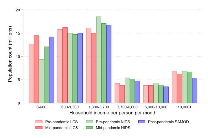
Our primary dataset is the Living Conditions Survey of 2014/5 (LCS 2015), which is a household
level survey with indicators of household income, housing, and education and health. In order to
appropriately cost and measure the impact of the grant scenarios, we update the 2014/5 Living
Conditions Survey (LCS) to more closely resemble the mid-pandemic environment as it was at the
end of 2020. We do this in three steps. Firstly, we forecast income to pre-pandemic levels using a
per capita growth in GDP from 2014 to 2019 of 17 per cent. Secondly, we reweight the dataset to
a) match 2020 demographics, disaggregated by race, age, gender and province, 12 and b) match the
administrative records on the taxable income distribution. Finally, we use the Quarterly Labour
Force Survey (QLFS) to calculate the change in employment from 2015 Q1 to 2020 Q1, and from
2020 Q1 to 2021 Q1, and implement these changes in the LCS dataset by randomly shocking
certain individuals from employment to unemployment, based on a set of demographic and
employment characteristics.
We can then recalculate the components of taxable income, market income, direct taxes and
contributions, and direct transfers so as to generate a new Disposable income aggregate for 2021.
Checking the decay in the Disposable income aggregate, we end up with a percentage change
9
It is expected that lags in data have incorrectly excluded high numbers of applicants in the existing implementation
of the Social Relief of Distress grant.
10
We explain this in detail in Sections 3.2.3 and Appendix B. Note that deciles are calculated based on household per
capita income, and so a child in a rich family, for example, will be in a higher decile despite earning zero individual
income.
11
An example of how this might work in practice, is that an EPWP programme with certain training targets is
incentivised to target individuals who are more easily trainable.
12
We do this using Wittenberg’s maxentropy package in Stata.
3decrease in Disposable income of 2.3 per cent, slightly higher than the percentage change decrease
in the GNI of 1.1 per cent and in the GDP of 2.0 per cent.
Table 1: Per capita growth in GNI, GDP, and Disposable income constructed within the LCS
Statistic / aggregate 2014/15 2019/20 Percentage 2020/21 Percentage
(R) (R) change (R) change
GNI 71 870 83 926 16.8 83 007 -1.1
GDP 73 690 86 375 17.2 84 606 -2.0
Disposable income (LCS) 41 175 47 763 16.0 46 675 -2.3
Source: authors' calculations based on LCS 2014/15, QLFS 2015 Q1, QLFS 2020 Q1, and QLFS 2021 Q1
Mean Disposable income decreases for all deciles from 2019/20 to 2020/21 except Decile 10
which sees a slight increase (Table 2).
Table 2: LCS Disposable income 2015, 2020, and 2021
Decile of Disposable income Percentage change
per capita (per capita, per month)
Disposable income
A. B. C. A to B B to C A to C
2014/15 2019/20 2020/21
1 170 209 199 22.7 -4.6 17.0
2 329 453 440 37.8 -2.8 33.9
3 474 652 621 37.4 -4.8 30.9
4 661 881 832 33.4 -5.7 25.9
5 915 1 173 1 093 28.1 -6.8 19.4
6 1 284 1 567 1 445 22.1 -7.8 12.6
7 1 899 2 253 2 049 18.6 -9.0 7.9
8 3 080 3 628 3 390 17.8 -6.6 10.1
9 5 970 7 062 6 752 18.3 -4.4 13.1
10 19 757 21 368 21 512 8.2 0.7 8.9
Total 3 454 3 925 3 835 13.6 -2.3 11.0
Note: the mean values per decile allow reranking such that columns are ranked by 2015, 2020 and 2021
Disposable income respectively.
Source: authors' calculations based on LCS 2014/15, QLFS 2015 Q1, QLFS 2020 Q1, and QLFS 2021 Q1.
Further details on this process, and a set of robustness checks, are included in Appendix A.
42.2 Methodology
We construct the scenarios on top of an existing model built for a 2014/15 Fiscal Incidence
analysis (CEQ Assessment). We improve on the previous version of the model for 2014/15 13 and
simultaneously update the instruments to match the 2020/21 policy environment and budget
numbers. 14
A flow chart which describes the construction of the CEQ Income Concepts from Market to
Disposable income is included below. We start at Market income, constructed using income from
private sources such as earnings from labour and capital, and grossed up by employer contributions
to the Unemployment Insurance Fund (UIF), Skills Development Levy (SDL), and the
Compensation Fund. We then subtract the direct taxes and contributions to generate Net market
income, and add in the value of social grants received, as well as near-cash transfers such as Free
Basic Services and housing subsidies to reach Disposable income. Disposable income is the
primary income concept we use for measuring poverty.
Note that for all of the expenditure scenarios which require means-testing, we construct an
aggregate which we call Observable income. The aggregate is designed to match what the
administrative authorities are able to measure. It overlaps with Disposable income, but excludes
the value of near-cash transfers, imputed rent 15 and remittances. It is only used to determine
means-tested programme eligibility; poverty is still measured using Disposable income.
Figure 1: Income concepts
Pre-fiscal = Market income
Wages and salaries, income from capital, retirement income, rent and imputed rent, alimony and
remittances, employer contributions to UIF, SDL & Compensation Fund.
- Direct taxes & contributions Net market income
Personal income tax; Contributions to UIF, SDL,
Compensation Fund
Observable income
Net Market Income + social grants -
imputed rent - remittances
+ Direct transfers
Social grants; Near-cash transfers (Free Basic Services,
housing subsidies) Disposable income
Source: adapted from Lustig (2018).
13
Deductions for retirement contributions and medical tax credits are more precisely modelled, and Market Income
is grossed upward to include employer contributions to the Compensation Fund, Unemployment Insurance Fund,
and Skills Development Levy.
14
Goldman, Woolard & Jellema (2020) describes the allocation methodology for each of the fiscal instruments, and
the income concepts, included here however the concepts shown in the original CEQ Assessment are based on the
official Statistics South Africa (Stats SA) consumption welfare aggregate, while here we based our Income Concepts
on an income aggregate.
15
Imputed rent is the rent a house owner would be willing to pay to live in their own house. It is included in the
income aggregates because 1) the additional money saved can be used to purchase other goods, thereby increasing the
purchasing power of a household to consume a basic basket of necessities and 2) the value of imputed rent can be
understood as a type of in-kind income the owner receives as a monthly return on their housing asset.
5In each subsection we present descriptive statistics regarding simulated programme costs,
coverage, and benefits. For coverage we show both the number of direct programme beneficiaries
and the sum of direct beneficiaries and ‘indirect’ beneficiaries (those co-resident with direct
beneficiaries). When showing benefits, we show the average per month value of the grant received
by direct beneficiaries.
In the analysis of each scenario, we refer to and draw from a set of indicators, which we define
here for ease of reference:
• Incidence: the ratio of total expenditures per decile to total income per decile.
• Concentration shares: the shares of total expenditure distributed to each decile.
• The impact of the grant on poverty reduction—using the poverty headcount ratio (per
cent of the population below the poverty line) and the poverty gap (the average
shortfall below the poverty line across the population, normalised by the poverty line).
• A measure of FPL spending efficiency: 16 the proportion of scenario spending which
contributes to a reduction in the FPL poverty gap.
We also use the term ‘Spillover’, in the paper, by which we refer to the spending which raises
previously poor households’ incomes over and above the poverty line.
In all cases, the baseline is Disposable income excluding the new scenario spending, and we
compare this with Disposable income including the new scenario spending. This allows the reader
to observe the Marginal impact on poverty reduction 17 of the simulated scenario. This also means that
the analysis we present here is explicitly about additions to the existing social grant system. We do
not analyse the impact of existing social grants, which we know already have a substantial impact
on poverty reduction. 18
2.3 Deciles, and national poverty lines
In order to better understand the information reported in the tables and graphs throughout this
paper, it is helpful to keep certain statistics in mind. The minimum, mean and maximum of
monthly per capita income at baseline Disposable income are shown for each decile in Table 3
below, and the values of the national poverty lines in Table 4. Note that all deciles are calculated
based on baseline Disposable per capita income.
16
Note that when we use efficiency here and throughout this paper, we are referring to what the CEQ Handbook
calls the Fiscal Gains to the Poor Effectiveness Indicator.
17
See Lustig (2018) for a discussion of Marginal impacts.
18
See, for example, Goldman, Woolard and Jellema (2020).
6Table 3: Minimum, mean, maximum per capita Disposable income per decile of Disposable income
Per capita monthly Disposable income
Decile Min Mean Max
1 - 199 347
2 347 440 530
3 530 621 719
4 719 832 955
5 955 1 093 1 248
6 1 248 1 445 1 684
7 1 684 2 049 2 546
8 2 546 3 390 4 486
9 4 486 6 743 10 170
10 10 170 21 488 164 066
Source: authors’ calculations based on LCS 2014/15, QLFS 2015 Q1, QLFS 2020 Q1, and QLFS 2021 Q1.
Putting this information together, we see that the FPL of R624 per month falls within the third
decile of baseline Disposable income, the LBPL falls within the fourth decile, and the UBPL falls
within the sixth decile.
Table 4: 2021 Poverty line values
Poverty line 2021 line values
Food Poverty Line (FPL) 624
Lower-bound Poverty Line (LBPL) 890
Upper-bound Poverty Line (UBPL) 1 335
Source: reproduced from Statistics South Africa (2021: 3, Table 1). 2021 line values are per person, per month.
3 Scenarios
This section first conducts a within-scenario comparison of each of the scenario variations, and
then chooses one variation to compare against the other scenarios in Section 4.
3.1 Child support grant
3.1.1 Description and methodology
In this scenario, the statutory Child Support Grant (CSG) amount is increased by 36 per cent from
R460 to the current FPL of R624 per month. 19 We simulate two variations on this scenario: The
first where the existing income threshold does not increase along with the grant value (i.e. R4600
19
The CSG values are based on reported values in the survey, which will make the results look less effective compared
to the other, simulated scenarios. We observe amounts received per caregiver not per child, and there are multiple
adults with children in each household, which complicates linking CSG recipient children within the household to
caregivers. We therefore back out the number of children by taking the value of the grant received and dividing by
the statutory amount for each household. We calculate the new CSG grant amount in the first variation, by multiplying
by 1.36 (the ratio of R624 and R460), and we calculate the CSG grant amount in the second variation by applying the
statutory amount multiplied by 2.0 - the average number of CSG recipient children per caregiver according to the
survey.
7per month 20 despite that the legislation provides for the CSG threshold to be the size of the grant
value multiplied by ten); and a second sub-scenario where the income threshold increases in line
with the new grant amount, to R6 240 per month. Of the existing social grants, the CSG reaches
by far the largest number of direct and indirect beneficiaries, and previous research has shown it
to be highly progressively targeted (Bassier et. al, 2021). Raising the value to the FPL is anticipated
to disproportionately benefit women and children, given the demographic structure of CSG-
receiving households.
3.1.2 Results
The average monthly value of the grant for beneficiaries increases from R458 to R623, with the
increased size of the grant, and the number of direct beneficiaries increases from 6.99 to 7.30
million when we raise the threshold to the R6240 required by the current regulations. The total
cost increases by R27.7 billion when we increase the size of the grant, and a further R4.7 billion
when we increase the threshold (Table 5).
Table 5: CSG value, beneficiaries, and total annual cost
Simulation Average monthly Total benef. Cost
value of grant (R) (millions) (R, billion)
Individual Direct Direct + Annual
Indirect
Baseline (R460, R4600) 458 6.99 30.0 76.8
Increased grant size (R624, R4600) 623 6.99 30.0 27.7
Increased size and threshold (R624, R6240) 624 7.30 30.8 32.4
Note: [1] given that we view caregivers and not children receiving the CSG, average monthly value of grant for
individuals is here the value of amount received by caregiver, divided by average of 2.0 children per caregiver. [2]
Grant values do not perfectly match statutory values because the baseline grant and first variation are based on
directly observed benefits in the dataset, rather than simulated values.
Source: authors’ calculations based on LCS 2014/15, QLFS 2015 Q1, QLFS 2020 Q1, and QLFS 2021 Q1.
Figure 2a and 2b show graphs of incidence and concentration for the CSG. A graph of incidence
shows the amount of grant expenditure provided to a particular decile, as a share of income earned
by the decile. It shows the benefit to an individual in that decile of a transfer and is a measure of
both size and distribution. Ultimately the incidence will explain graphically why we are seeing a
particular poverty impact. We also show the concentration shares, which show the percentage of
the transfer going to each decile, abstracted from programme size. The concentration shares are
also an absolute measure of distribution - they are not relative to income. Comparing concentration
shares with income is particularly useful for understanding the efficiency results and can (roughly)
tell us whether a transfer is progressive relative to income.
In Figure 2b the baseline and variation with increased grant size are perfectly overlaid, meaning
that increasing the size of the CSG does not change its distribution across the deciles. This is
because increasing the size of the CSG results in the same factor increase in the grant amount for
all recipients. Once we add the additional spending above the current threshold, however, richer
households become eligible for the grant. The grant becomes less pro-poor, as a result, with
20
The threshold is actually implemented as R4600 for a single individual, and R9200 for a married couple. For
simplification we only report the single threshold here, but we retain the ratio of 2:1 size of the income threshold for
married couples and single individuals.
8Deciles 1-6 receiving a slightly smaller share of total disbursements, and Deciles 7-10 receiving a
larger share.
Note also that the share of new CSG expenditure appears lower in Decile 1 than in Deciles 2 and
above at Disposable income (Figure 2b). This is purely because the Disposable income measure
already includes the baseline CSG measure, and thus a substantial amount of reranking has
occurred - by which we mean that a number of households which were in Decile 1 have moved
to higher deciles because of the CSG receipt. Comparing the same graph ranked by Market income
(prior to the inclusion of the baseline CSG), the results show roughly equal shares of CSG
expenditure going to Deciles 1 and 2.
In all three variants, the incidence of the grant becomes smaller as we move towards the richer
end of the distribution. This is partly because the grant values are smaller as a share of income for
the upper deciles, and partly because there are fewer recipients.
Increasing the grant size increases the incidence across all deciles, as there is no change to numbers
of recipients, only to grant size. Raising the threshold, however, has no impact on the incidence in
deciles 1-3 21 (Figure 2a) as the additional expenditure all goes to individuals above the threshold.
Figure 2: Child support grant a. Incidence (top panel), b. Concentration shares (bottom panel)
80
Disposable income
Share of baseline
60
CSG base
40
CSG Increased grant size (R624,
20 R4600)
CSG Increased size and
-
threshold (R624, R6240)
1 2 3 4 5 6 7 8 9 10
Decile of baseline Disposable income
20
Per cent of transfer
15
CSG baseline
10
Increased grant size top-up (R624,
5 R4600)
Increased size and threshold top-
0
up (R624, R6240)
1 2 3 4 5 6 7 8 9 10
Decile of (baseline) Disposable income
Note: poverty is measured at Disposable income.
Source: authors’ calculations based on the LCS 2014/15, QLFS 2020 Q1, and QLFS 2020 Q2.
Figure 3a shows the impact on poverty of a particular variation. The first bar shows the size of the
baseline FPL Poverty Headcount and Poverty Gap, and the second and third bars show the scenario
FPL poverty headcount and gap. By comparing the size of the FPL Poverty Gap at the baseline
21
Only in deciles 6-8 are the increases greater than 0.4 percent of income per decile and range from 0.4 to 1 percent
9(10.2 per cent) with the FPL Poverty Gap after the introduction of the Increased grant size (8.3
per cent), we can determine that the marginal contribution of the CSG Increased grant size top-
up to FPL poverty gap reduction is 1.8 percentage points (10.16 – 8.33) - another way of saying
that is the poverty gap is reduced by 1.8 percentage points.
Figure 3b shows the FPL efficiency scores 22 of the two top-ups, both combined with the original
CSG and on their own. This measure calculates the expenditure that goes to topping the baseline
Disposable income of the poor up to the FPL, but not including any Spillover, as a share of total
grant expenditure. In 3b we show the efficiency measure of the CSG at the baseline for comparison
with the top-ups, as well as, for completeness, the efficiency of the total grant once the top-ups
are combined with the baseline. 23
From the zero additional incidence in Deciles 1-3 for the second variation (Figure 2a), we can
know that none of the grant expenditure is going to those households with income lower than the
FPL. As a result, the efficiency of the second top-up in Figure 3b is zero. Expenditures used to
top up the CSG size are less efficient than the baseline CSG at 29.5 per cent. This is because, once
the baseline CSG is already included, the top-up is more likely to result in Spillover. 24
The increased grant size CSG top-up reduces the FPL poverty headcount and gap by 3.3
percentage points and 1.8 percentage points respectively, while increasing the eligibility threshold
results in no additional poverty reduction impact at the FPL (Figure 3a) given that no expenditure
reaches deciles 1-3.
22
As described in Section 2.2., by efficiency we mean the percentage of grant expenditure that goes to reducing the
FPL gap.
23
Note that for the cumulative measures this is calculated as the share of CSG expenditure that goes to those
individuals who are poor, as measured by their Disposable income less baseline CSG expenditure, and which tops
them up to the FPL poverty line, as a share of total CSG expenditure. For the top-up measures, we measure income
by Disposable income plus baseline CSG expenditure.
24
In Decile 2, 160 thousand individuals that are poor in the baseline scenario, are now above the FPL once the grant
size is increased. In Decile 3, there are 1.6 million additional individuals over the FPL.
10Figure 3: a. Poverty reduction (LHS panel), and b. FPL Efficiency (RHS panel).
43.9
25.3
40.1
38.3
Per cent of spending reducing FPL gap
22.0
Baseline
29.5
25.2
Per cent
CSG Increased
grant size (R624,
R4600)
10.2
8.3
CSG Increased
size and
threshold (R624,
R6240) -
CSG CSG with CSG with Increased Inreased Increased
Baseline increased increased grant size size and threshold
(R460, size (R624, size and top-up threshold top-up
FPL FPL gap R4600) R4600) threshold
(R624,
top-up
headcount R6240)
Note: [1] poverty is measured at Disposable income. [2] For the grant which include the baseline CSG grant only,
efficiency is calculated as the share of CSG expenditure that i) goes to those individuals who are poor, as
measured by their Disposable income without the CSG, and ii) which tops them up to (but not above) the FPL
poverty line, as a share of total CSG expenditure.
Source: authors’ calculations based on the LCS 2014/15, QLFS 2020 Q1, and QLFS 2020 Q2.
It is not surprising that increasing the size of the CSG (an already very effective grant) reduces its
efficiency at the FPL, as it now brings individuals (further) above the poverty line. However, an
increase in the size of the CSG pay-out, at a cost of R27.7 billion, is relatively easy to implement,
and as noted above it disproportionately benefits women and children. On the other hand, it does
not significantly expand the social safety net to include new individuals, and using a grant designed
to target children for a more general expansion of the safety net would mean relying on indirect
targeting of other population groups and would exclude poor households without children. In
Section 4 we show how the topping-up of the CSG without changing its eligibility threshold
performs against the alternative scenarios, given the negligible benefit at the FPL of raising the
threshold.
3.2 Special COVID-19 Social Relief of Distress
3.2.1 Description and methodology
This scenario largely mimics the Special COVID-19 Social Relief of Distress (SRD) grant—a R350
grant currently provided by the Department of Social Development. While the design of the grant
was ostensibly targeting those with no means of supporting themselves, in reality the grant was
provided to those whose status was deemed to be not formally employed, with a means test applied
only for those individuals who appealed their grant denial. It was first introduced in May 2020 and
has since been extended three times, with the latest extension until March 2022. There have been
various calls to make the grant permanent.
11In the modelled scenario, the default grant is provided to all those aged 18-59 who are not formally
employed 25, and not receiving any other social grant income (except the CSG, foster child grant
or care dependency grant). Only the formally employed are excluded because the state does not
have records of informal employment to exclude these workers, and they may face increased
labour market precarity in any case. In some variants we impose additional individual income
means tests, or vary the age restriction. The actual experience of SRD roll-out has been that many
fewer people receive the SRD than are eligible in the survey data. This is discussed in Section 3.2.3.
We include in our scenarios a ‘scaled-down’ version of the SRD, where we randomly select eligible
individuals up to a population of 9.5 million SRD recipients, to match the maximum number
currently budgeted for. 26 Note that the take-up rate directly impacts the cost of the grant; the full
take-up and scaled down versions may be interpreted as bounds on the actual cost (the scaled
down variation is 45 per cent of the cost of the full-take up variation). Similar considerations apply
to the costing of the other variations.
The scenario includes the following specific variations:
i. SRD full take up: R350, as described (no scaling, no income threshold);
ii. Emergency: R350, recipients scaled down to reach 9.5 million (designed to replicate
the current number of recipients);
iii. Job seekers: R350, no scaling, but restricted to age 18-34;
iv. FPL threshold: R350 with the additional eligibility criterion of individual observable
income (if any) being less than R624 per month;
v. NMW threshold: R350 with the additional eligibility criterion of individual reported
income (if any) being less than R3 570 per month (the national minimum wage);
vi. SRD 624 NMW threshold: as above with NMW threshold, but with increased value of
grant to FPL (R624 per month).
Note that we do not apply an income threshold in scenarios i through iii, as we aim to replicate
how the grant was actually administered, rather than how it was originally conceived.
3.2.2 Results
The number of recipients, and therefore the cost, changes substantially in the different variations
of the SRD (Table 6). The full-take up scenario provides an SRD grant directly to 21.5 million
individuals. Given that no means test is applied in this scenario, there are 1.6 million not formally
employed working age individuals with income (not from formal employment) above the National
Minimum Wage who are nonetheless eligible for the grant. At the NMW threshold, in which 19.9
million individuals are directly eligible for a grant. We model two variants of this—one at the R350
grant size, and one at the size of the FPL of R624. Implementing a lower threshold, at the FPL,
reduces the number of recipients to 16.8 million, and restricting to adults age 18-34 (young ‘job-
seekers’) further curbs the numbers to 13.4 million. In the ‘emergency’ variant we restrict the SRD
recipients to 9.5 million (again with no income threshold), as noted above, and finally the SRD
with the FPL threshold implemented together with the CSG top-up (not shown here) reaches 19.9
25
One significant limitation of the LCS data is that it reports on the formal/informal sector of work, but not on
whether the work itself is formal or informal (some people have informal employment in the formal sector). It also
does not contain any variables which would allow us to infer work status (such as whether or not the respondent has
a work contract, and benefits from paid annual leave). We use the formal sector as a proxy for informal employment
in general.
26
We call this the ‘emergency’ scenario, to reflect that limited receipt may be partly caused by the short timeframe of
current SRD implementation, which affects both the number of applications and the accuracy of the approval process.
12direct beneficiaries. In all variations, beneficiaries receive a value of R350 except for variation (iii)
where we increase the size of the grant to R624.
Table 6: SRD value, beneficiaries, and total annual cost
Variation Average value Total beneficiaries Annual cost
(millions)
Individual, per month Direct Indirect (R, billion)
Full take-up 350 21.5 48.7 90.3
NMW threshold 350 19.9 46.7 83.7
R624 at NMW threshold 624 19.9 46.7 149.2
FPL threshold 350 16.8 43.0 70.6
Youth / job-seekers 350 13.4 38.8 56.2
Emergency 350 9.5 31.8 39.9
Source: authors’ calculations based on LCS 2014/15, QLFS 2015 Q1, QLFS 2020 Q1, and QLFS 2021 Q1.
All variations on the SRD have a similar distribution, in terms of the share of the total which goes
to each decile (Figure 4b), however the incidence per decile varies with the number of beneficiaries
within the decile receiving the grant (Figure 4a). For example, the NMW threshold variation results
in a benefit for the first decile to the size of 180 per cent of total baseline Disposable income in
Decile 1, while the Emergency variation provides a benefit of only 48 per cent.
The variation which provides R624 per beneficiary, with a threshold at the NMW provides the
largest disbursement for Deciles 1-3 (Figure 4a). It therefore reduces FPL poverty significantly
more than the other variations. The headcount index drops to 8.9 per cent (16.4 p.p. reduction)
and the poverty gap to 1.8 per cent (8.3 p.p. reduction) (Figure 5a). It costs R149.2 billion - more
than double the variation with an FPL threshold and a R350 grant value (Table 6). Unsurprisingly,
this variation is the least efficient at FPL poverty reduction in terms of share of expenditure which
reduces the FPL gap (Figure 5b). Given that the size of the grant is larger, it is more likely to create
Spillover above the FPL than the other variations, and the eligibility threshold is higher than the
FPL, resulting in larger income increases for households above the FPL (mainly Deciles 4-10 27).
The concentration shares are exactly the same as for the R350 variation with the NMW threshold
(Figure 4b).
The SRD at full take-up costs slightly more (at R91.2 billion) than the variation with a NMW
threshold and with a R350 grant, and yet has almost identical incidence in Deciles 1-3 (It is not
visible in Figure 4a, covered by the NMW variation). It therefore has the same impact on the
poverty headcount and poverty gap (reducing the headcount to 17.3 per cent, and the poverty gap
to 4.5 per cent, Figure 4a). This is unsurprising because any individual excluded from the SRD by
the NMW threshold already lives in a household with a per capita Disposable income greater than
the FPL, and so the two policies reduce poverty to the same extent. However, the NMW threshold
does ensure some high-income individuals are excluded from SRD eligibility, thus reducing the
programme’s budget and improving its efficiency (28.2 for full take-up SRD versus 30.4 for the
NMW threshold variation, Figure 5b).
27
There are increases in Deciles 8 to 10, although not visible on the graph.
13Figure 4: Social Relief of Distress a. Incidence (top panel), b. Concentration shares (bottom panel)
200
Share of baseline Disposable income
180
160
140 Full take-up
120
Emergency
100
Youth
80
FPL threshold
60
40 NMW threshold (R350)
20 NMW threshold (R624)
0
1 2 3 4 5 6 7 8 9 10
Decile of baseline Disposable income
25
20
Per cent of transfer
15 Full take-up
Emergency
10 Youth
FPL threshold
5
NMW threshold (R350 & R624)
0
1 2 3 4 5 6 7 8 9 10
Decile of baseline Disposable income
Note: poverty is measured at Disposable income.
Source: authors’ calculations based on the LCS 2014/15, QLFS 2020 Q1, and QLFS 2020 Q2.
The variation with a means-test cut-off at the FPL, has a (barely discernible) lower incidence in
Deciles 1-3 than the full take-up and NMW variations, and therefore the remaining poverty is
slightly higher at 18.0 per cent headcount, 4.6 per cent FPL gap. Nonetheless, it directs a larger
share of total expenditures to the poorest decile (Figure 4b), and so scores higher on the FPL
Efficiency measure (the higher the threshold is above the FPL, the more likely we are to include
individuals with a per capita income above the FPL).
The ‘emergency’ SRD, scaled down to 9.5 million beneficiaries, and the youth SRD, limited to ages
18-35, have the lowest marginal impact on poverty reduction. This is because they have the
smallest incidence in Deciles 1-7 of all the variations. Nonetheless, they are still fairly effective in
terms of the proportion of expenditure targeting the FPL, with only the FPL threshold variation
scoring higher in terms of efficiency, and the youth variation scoring similarly to the NMW
threshold variation. This result can be understood by examining the average value of grant received
per beneficiary household, not shown here. Households receiving at least one SRD grant in the
full take-up variation, for example, receive on average R625 per household (as there is an average
of 1.8 SRD recipients per household). In the emergency scenario, however, households receive on
average R477 per household (an average of 1.4 recipients per household). The full take-up SRD
will therefore result in more Spillover for households than the emergency SRD.
Given its relatively high efficiency, we choose the R350 SRD with the FPL threshold to compare
with the alternative scenarios in Section 4.
14Figure 5: SRD a. Poverty reduction and b. FPL Efficiency
35.1
Per cent of sepdning reducing FPL poverty gap
32.2
30.4 30.4 30.3
25.3 28.2
21.3 24.9
20.3
Baseline
18.0
SRD - scaled down
SRD-job-seekers
Per cent
17.3
SRD - FPL
SRD
10.2
SRD - NMW
7.3 SRD624 - NMW
8.9
6.4
4.6
4.5
1.8
FPL headcount FPL gap
Note: poverty is measured at Disposable income.
Source: authors’ calculations based on the LCS 2014/15, QLFS 2020 Q1, and QLFS 2020 Q2.
3.2.3 Current SRD implementation
The substantial implementation difficulties associated with the current SRD roll-out are detailed
in Appendix B, based on meetings with SASSA officials. They give rise to a concern that we may
be overstating the efficiency of the SRD. The relevance of these difficulties for our analysis will
depend on whether we believe that a future SRD grant implemented as a medium to long-term
policy option is likely to be plagued by the same challenges as an SRD grant implemented in the
midst of a pandemic, and whether these challenges are particular to an SRD type grant or are likely
to be faced across all scenarios.
As a result of the lags in employment verification, combined with very high rates of labour market
churn in South Africa (especially so during the pandemic), an extremely large proportion of eligible
SRD applicants are likely to be incorrectly rejected from grant receipt. Our preferred estimate is
that the proportion of false rejections is close to 15 per cent, and not larger than 30 per cent.
There are reasons that our approximate estimates of false rejections may be overestimated or
underestimated, and further investigation into SASSA’s verification systems would allow a more
precise figure. We arrive at this estimate via two methods, one based on compounding observed
short-term (3-month) rates in labour market churn from the Quarterly Labour Force Survey, and
the second considering the actual rejection rates published by SASSA for the August 2021 SRD
applications.
Using the first method, compounding observed short-term rates in labour market churn, we
estimate that about one third of eligible applicants could be rejected because their employment
status is tested against outdated administrative databases, with employment as long as 18 months
before the time of application sometimes liable to cause rejection. There are a number of caveats
association with this result. Firstly, extrapolating short-term (3 month) churning rates back 18
months is likely to overestimate labour market transitions and false rejections, as the long-term
15You can also read