SMOOTH MARKETS: A BASIC MECHANISM FOR ORGANIZING GRADIENT-BASED LEARNERS
←
→
Page content transcription
If your browser does not render page correctly, please read the page content below
Published as a conference paper at ICLR 2020

                                          S MOOTH MARKETS : A BASIC MECHANISM FOR
                                          ORGANIZING GRADIENT- BASED LEARNERS

                                           David Balduzzi1 , Wojciech M Czarnecki1 , Thomas W Anthony1 , Ian M Gemp1 ,
                                           Edward Hughes1 , Joel Z Leibo1 , Georgios Piliouras2 , Thore Graepel1
                                           1
                                             DeepMind ; 2 Singapore University of Technology and Design
                                           {dbalduzzi,lejlot,twa,imgemp,edwardhughes,jzl,georgios,thore}@∗

                                                                                        A BSTRACT
arXiv:2001.04678v2 [cs.LG] 18 Jan 2020

                                                   With the success of modern machine learning, it is becoming increasingly important
                                                   to understand and control how learning algorithms interact. Unfortunately, negative
                                                   results from game theory show there is little hope of understanding or controlling
                                                   general n-player games. We therefore introduce smooth markets (SM-games), a
                                                   class of n-player games with pairwise zero sum interactions. SM-games codify a
                                                   common design pattern in machine learning that includes (some) GANs, adversarial
                                                   training, and other recent algorithms. We show that SM-games are amenable to
                                                   analysis and optimization using first-order methods.

                                         “I began to see legibility as a central problem in modern statecraft. The premodern state was, in many
                                          respects, partially blind [. . .] It lacked anything like a detailed ‘map’ of its terrain and its people. It
                                          lacked, for the most part, a measure, a metric that would allow it to ‘translate’ what it knew into a
                                          common standard necessary for a synoptic view. As a result, its interventions were often crude and
                                          self-defeating.”
                                         – from Seeing like a State by Scott (1999)

                                          1     I NTRODUCTION

                                         As artificial agents proliferate, it is increasingly important to analyze, predict and control their
                                         collective behavior (Parkes and Wellman, 2015; Rahwan et al., 2019). Unfortunately, despite almost a
                                         century of intense research since von Neumann (1928), game theory provides little guidance outside a
                                         few special cases such as two-player zero-sum, auctions, and potential games (Monderer and Shapley,
                                         1996; Nisan et al., 2007; Vickrey, 1961; von Neumann and Morgenstern, 1944). Nash equilibria
                                         provide a general solution concept, but are intractable in almost all cases for many different reasons
                                         (Babichenko, 2016; Daskalakis et al., 2009; Hart and Mas-Colell, 2003). These and other negative
                                         results (Palaiopanos et al., 2017) suggest that understanding and controlling societies of artificial
                                         agents is near hopeless. Nevertheless, human societies – of billions of agents – manage to organize
                                         themselves reasonably well and mostly progress with time, suggesting game theory is missing some
                                         fundamental organizing principles.
                                          In this paper, we investigate how markets structure the behavior of agents. Market mechanisms
                                          have been studied extensively (Nisan et al., 2007). However, prior work has restricted to concrete
                                          examples, such as auctions and prediction markets, and strong assumptions, such as convexity. Our
                                          approach is more abstract and more directly suited to modern machine learning where the building
                                          blocks are neural nets. Markets, for us, encompass discriminators and generators trading errors in
                                          GANs (Goodfellow et al., 2014) and agents trading wins and losses in StarCraft (Vinyals et al., 2019).

                                          1.1   OVERVIEW

                                         The paper introduces a class of games where optimization and aggregation make sense. The phrase
                                         requires unpacking. “Optimization” means gradient-based methods. Gradient descent (and friends)
                                         are the workhorse of modern machine learning. Even when gradients are not available, gradient
                                         estimates underpin many reinforcement learning and evolutionary algorithms. “Aggregation” means
                                         weighted sums. Sums and averages are the workhorses for analyzing ensembles and populations

                                                                                               1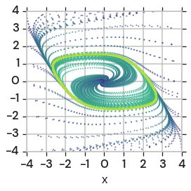
Published as a conference paper at ICLR 2020

across many fields. “Makes sense” means we can draw conclusions about the gradient-based dynamics
of the collective by summing over properties of its members.
As motivation, we present some pathologies that arise in even the simplest smooth games. Examples in
section 2 show that coupling strongly concave profit functions to form a game can lead to uncontrolled
behavior, such as spiraling to infinity and excessive sensitivity to learning rates. Hence, one of our
goals is to understand how to ‘glue together agents’ such that their collective behavior is predictable.
Section 3 introduces a class of games where simultaneous gradient ascent behaves well and is
amenable to analysis. In a smooth market (SM-game), each player’s profit is composed of a
personal objective and pairwise zero-sum interactions with other players. Zero-sum interactions are
analogous to monetary exchange (my expenditure is your revenue), double-entry bookkeeping (credits
balance debits), and conservation of energy (actions cause equal and opposite reactions). SM-games
explicitly account for externalities. Remarkably, building this simple bookkeeping mechanism into
games has strong implications for the dynamics of gradient-based learners. SM-games generalize
adversarial games (Cai et al., 2016) and codify a common design pattern in machine learning, see
section 3.1.
Section 4 studies SM-games from two points of view. Firstly, from that of a rational, profit-maximizing
agent that makes decisions based on first-order profit forecasts. Secondly, from that of the game as a
whole. SM-games are not potential games, so the game does not optimize any single function. A
collective of profit-maximizing agents is not rational because they do not optimize a shared objective
(Drexler, 2019). We therefore introduce the notion of legibility, which quantifies how the dynamics
of the collective relate to that of individual agents.
Finally, section 5 applies legibility to prove some basic theorems on the dynamics of SM-games under
gradient-ascent. We show that (i) Nash equilibria are stable; (ii) that if profits are strictly concave
then gradient ascent converges to a Nash equilibrium for all learning rates; and (iii) the dynamics are
bounded under reasonable assumptions.
The results are important for two reasons. Firstly, we identify a class of games whose dynamics are,
at least in some respects, amenable to analysis and control. The kinds of pathologies described in
section 2 cannot arise in SM-games. Secondly, we identify the specific quantities, forecasts, that are
useful to track at the level of individual firms and can be meaningfully aggregated to draw conclusions
about their global dynamics. It follows that forecasts should be a useful lever for mechanism design.

1.2   R ELATED WORK

A wide variety of machine learning markets and agent-based economies have been proposed and
studied: Abernethy and Frongillo (2011); Balduzzi (2014); Barto et al. (1983); Baum (1999); Hu
and Storkey (2014); Kakade et al. (2003; 2005); Kearns et al. (2001); Kwee et al. (2001); Lay and
Barbu (2010); Minsky (1986); Selfridge (1958); Storkey (2011); Storkey et al. (2012); Sutton et al.
(2011); Wellman and Wurman (1998). The goal of this paper is different. Rather than propose another
market mechanism, we abstract an existing design pattern and elucidate some of its consequences for
interacting agents.
Our approach draws on work studying convergence in generative adversarial networks (Balduzzi
et al., 2018; Gemp and Mahadevan, 2018; Gidel et al., 2019; Mescheder, 2018; Mescheder et al.,
2017), related minimax problems (Abernethy et al., 2019; Bailey and Piliouras, 2018), and monotone
games (Gemp and Mahadevan, 2017; Nemirovski et al., 2010; Tatarenko and Kamgarpour, 2019).

1.3   C AVEAT

We consider dynamics in continuous time dw    dt = ξ(w) in this paper. Discrete dynamics, wt+1 ←
wt + ξ(w) require a more delicate analysis, e.g. Bailey et al. (2019). In particular, we do not claim
that optimizing GANs and SM-games is easy in discrete time. Rather, our analyis shows that it is
relatively easy in continuous time, and therefore possible in discrete time, with some additional effort.
The contrast is with smooth games in general, where gradient-based methods have essentially no
hope of finding local Nash equilibria even in continuous time.

                                                   2
Published as a conference paper at ICLR 2020
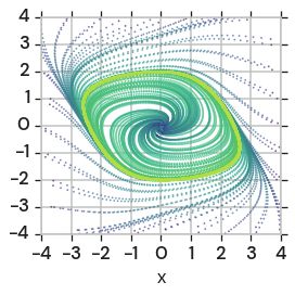
A η1 = η2 B η1 = η2
C D
η1 = η2 ⁄ 8 η1 = η2 ⁄ 8
half a game minimal NZ
Figure 1: Effect of learning rates in two games. Note: x-axis is log-scale. Left: “half a game”,
e.g. 2. Right: minimal SM-game, e.g. 3. Top: Both players have same learning rate. Bottom: Second
player has 18 learning rate of first (which is same as for top). Reducing the learning rate of the second
player destabilizes the dynamics in “half a game”, whereas the SM-game is essentially unaffected.
1.4 N OTATION
Vectors are column-vectors. The notations S 0 and v 0 refer to a positive-definite matrix and
vector with all entries positive respectively. Rather than losses, we work with profits. Proofs are in
the appendix. We use economic terminology (firms, profits, forecasts, and sentiment) even though the
examples of SM-games, such as GANs and adversarial training, are taken from mainstream machine
learning. We hope the economic terminology provides an invigorating change of perspective. The
underlying mathematics is no more than first and second-order derivatives.
profit of firm i πi (w) (1)
gradient of profit ξ i (w) := ∇wi πi (w)
|
profit forecast fPvi (w) := vi · ξ i (w) (2)
aggregate forecast i fvi (wi ) (3)
sentiment of firm i vi| · ∇wi fvi (w) (4)
2 S MOOTH GAMES
Smooth games model interacting agents with differentiable objectives. They are the kind of games
that are played by neural nets. In practice, the differentiability assumption can be relaxed by replacing
gradients with gradient estimates.
Definition 1. A smooth game (Letcher et al., 2019) consists in n players [n] = {1, . . . , n}, equipped
with twice continuously differentiable profit functions
Pn {πi : Rd → R}ni=1 . The parameters are
d di
w = (w1 , . . . , wn ) ∈ R with wi ∈ R where i=1 di = d. Player i controls the parameters wi .
If players update their actions via simultaneous gradient ascent, then a smooth game yields a
dynamical system specified by the differential equation dw
dt = ξ(w) for
ξ(w) := ξ 1 (w), . . . , ξ n (w)
where ξ i (w) := ∇wi πi (w) is a di -vector. The Jacobian of a game is the (d × d)-matrix of second-
d
derivatives J(w) := ∂ξ∂w α (w)
β
. The setup can be recast in terms of minimizing losses by
α,β=1
substituting `i := −πi for all i.
Smooth games are too general to be tractable since they encompass all dynamical systems.
Lemma 1. Every continuous dynamical system on Rd , for any d, arises as simultaneous gradient
ascent on the profit functions of a smooth game.
The next two sections illustrate some problems that arise in simple smooth games.
Definition 2. We recall some solution concepts from dynamical systems and game theory:
3Published as a conference paper at ICLR 2020
• A stable fixed point1 w∗ satisfies ξ(w∗ ) = 0 and v| · J(w∗ ) · v < 0 for all vectors v 6= 0.
• A local Nash equilibrium w∗ has neighborhoods Ui of wi∗ for all i, such that
∗
πi (wi , w−i ) < πi (wi∗ , w−i
∗
) all wi ∈ Ui \ {wi∗ }.
• A classical Nash equilibrium w∗ satisfies πi (wi , w−i
∗
) ≤ πi (wi∗ , w−i
∗
) for all wi and all
players i.
Example 1 below shows that stable fixed points and local Nash equilibria do not necessarily coincide.
The notion of classical Nash equilibrium is ill-suited to nonconcave settings.
Intuitively, a fixed point is stable if all trajectories sufficiently nearby flow into it. A joint strategy is a
local Nash if each player is harmed if it makes a small unilateral deviation. Local Nash differs from
the classic definition in two ways. It is weaker, because it only allows small unilateral deviations.
This is necessary since players are neural networks and profits are not usually concave. It is also
stronger, because unilateral deviations decrease (rather than not increase) profits.
2.1 P ROBLEMS WITH POTENTIAL GAMES
A game is a potential game if ξ = ∇φ for some function φ, see Balduzzi et al. (2018) for details.
Example 1 (potential game). Fix a small > 0. Consider the two-player games with profit functions
π1 (w) = w1 w2 − w12 and π2 (w) = w1 w2 − w22 .
2 2
The game has a unique local Nash equilibrium at w = (0, 0) with π1 (0, 0) = 0 = π2 (0, 0).
The game is chosen to be as nice as possible: π1 and π2 are strongly concave functions of w1
and w2 respectively. The game is a potential game since ξ = (w2 − w1 , w1 − w2 ) = ∇φ for
φ(w) = w1 w2 − 2 (w12 + w22 ). Nevertheless, the game exhibits three related problems.
Firstly, the Nash equilibrium is unstable. Players at the Nash equilibrium can increase their profits
via the joint update w ← (0, 0) + η · (1, 1), so π1 (w) = η(1 − 2 ) = π2 (w) > 0. The existence
of a Nash equilibrium where players can improve their payoffs by coordinated action suggests the
incentives are not well-designed.
Secondly, the dynamics can diverge to infinity. Starting at w(1) = (1, 1) and applying simultaneously
gradient ascent causes the norm of vector kw(t) k2 to increase without limit as t → ∞ – and at
an accelerating rate – due to a positive feedback loop between the players’ parameters and profits.
Finally, players impose externalities on each other. The decisions of the first player affect the profits
of the second, and vice versa. Obviously players must interact for a game to be interesting. However,
positive feedback loops arise because the interactions are not properly accounted for.
In short, simultaneous gradient ascent does not converge to the Nash – and can diverge to infinity. It
is open to debate whether the fault lies with gradients, the concept of Nash, or the game structure. In
this paper, we take gradients and Nash equilibria as given and seek to design better games.
2.2 P ROBLEMS WITH LEARNING RATES
Gradient-based optimizers rarely follow the actual gradient. For example RMSProp and Adam use
adaptive, parameter-dependent learning rates. This is not a problem when optimizing a function.
Suppose f (w) is optimized with reweighted gradient (∇f )η := (η1 ∇1 f, . . . , ηn ∇n f ) where η 0
is a vector of learning rates. Even though (∇f )η is not necessarily the gradient of any function, it
behaves like ∇f because they have positive inner product when ∇f 6= 0:
X
(∇f )|η · ∇f = ηi · (∇i f )2 > 0, since ηi > 0 for all i.
i
Parameter-dependent learning rates thus behave well in potential games where the dynamics derive
from an implicit potential function ξ(w) = ∇φ(w). Severe problems can arise in general games.
1
Berard et al. (2019) use a different notion of stable fixed point that requires J has positive eigenvalues.
4Published as a conference paper at ICLR 2020
Example 2 (“half a game”). Consider the following game, where the w2 -player is indifferent to w1 :
π1 (w) = w1 w2 − w12 and π2 (w) = − w22 .
2 2
The dynamics are clear by inspection: the w2 -player converges to w2 = 0, and then the w1 -player
does the same. It is hard to imagine that anything could go wrong. In contrast, behavior in the next
example should be worse because convergence is slowed down by cycling around the Nash:
Example 3 (minimal SM-game). A simple SM-game, see definition 3, is
π1 (w) = w1 w2 − w12 and π2 (w) = −w1 w2 − w22 .
2 2
Figure 1 shows the dynamics of the games, in discrete time, with small learning rates and small
gradient noise. In the top panel, both players have the same learning rate. Both games converge.
Example 2 converges faster – as expected – without cycling around the Nash.
In the bottom panels, the learning rate of the second player is decreased by a factor of eight. The
SM-game’s dynamics do not change significantly. In contrast, the dynamics of example 2 become
unstable: although player 1 is attracted to the Nash, it is extremely sensitive to noise and does not
stay there for long. One goal of the paper is to explain why SM-games are more robust, in general, to
differences in relative learning rates.
2.3 S T O P G R A D I E N T AND LEARNING RATES
Tools for automatic differentiation (AD) such as TensorFlow and PyTorch include stop gradient
operators that stop gradients from being computed. For example, let f (w) = w1 ·
stop gradient(w2 ) − 2 (w12 + w22 ). The use of stop gradient means f is not strictly
speaking a function and so we use ∇AD to refer to its gradient under automatic differentiation.
Then
∇AD f (w) = (w2 − w1 , −w2 )
which is the simultaneous gradient from example 2. Any smooth vector field is the gradient of a
function augmented with stop gradient operators, see appendix D. Stop gradient is often
used in complex neural architectures (for example when one neural network is fed into another
leading to multiplicative interactions), and is thought to be mostly harmless. Section 2.2 shows that
stop gradients can interact in unexpected ways with parameter-dependent learning rates.
2.4 S UMMARY
It is natural to expect individually well-behaved agents to also behave well collectively. Unfortunately,
this basic requirement fails in even the simplest examples.
Maximizing a strongly concave function is well-behaved: there is a unique, finite global maximum.
However, example 1 shows that coupling concave functions can cause simultaneous gradient ascent
to diverge to infinity. The dynamics of the game differs in kind from the dynamics of the players
in isolation. Example 2 shows that reducing the learning rate of a well-behaved (strongly concave)
player in a simple game destabilizes the dynamics. How collectives behave is sensitive not only to
profits, but also to relative learning rates. Off-the-shelf optimizers such as Adam (Kingma and Ba,
2015) modify learning rates under the hood, which may destabilize some games.
3 S MOOTH M ARKETS (SM- GAMES )
Let us restrict to more structured games. Take an accountant’s view of the world, where the only
thing we track is the flow of money. Interactions are pairwise. Money is neither created nor destroyed,
so interactions are zero-sum. If we model the interactions between players by differentiable functions
gij (wi , wj ) that depend on their respective strategies then we have an SM-game. All interactions
are explicitly tracked. There are no externalities off the books. Positive interactions, gij > 0, are
revenue, negative are costs, and the difference is profit. The model prescribes that all firms are profit
maximizers. More formally:
5Published as a conference paper at ICLR 2020
Definition 3 (SM-game). A smooth market is a smooth game where interactions between players
are pairwise zero-sum. The profits have the form
X
πi (w) = fi (wi ) + gij (wi , wj ) (1)
j6=i
where gij (wi , wj ) + gji (wj , wi ) ≡ 0 for all i, j.
The functions fi can act as regularizers. Alternatively, they can be interpreted as natural resources or
dummy players that react too slowly to model as players. Dummy players provide firms with easy
(non-adversarial) sources of revenue.
Humans, unlike firms, are not profit-maximizers; humans typically buy goods because they value
them more than the money they spend on them. Appendix C briefly discusses extending the model.
3.1 E XAMPLES OF SM- GAMES
SM-games codify a common design pattern:
1. Optimizing a function. A near-trivial case is where there is a single player with profit
π1 (w) = f1 (w).
2. Generative adversarial networks and related architectures like CycleGANs are zero or near
zero sum (Goodfellow et al., 2014; Wu et al., 2019; Zhu et al., 2017).
3. Zero-sum polymatrix games are SM-games where fi (wi ) ≡ 0 and gij (wi , wj ) =
wi| Aij wj for some matrices Aij . Weights are constrained to probability simplices. The
games have nice properties including: Nash equilibria are computed via a linear program
and correlated equilibria marginalize onto Nash equilibria (Cai et al., 2016).
4. Intrinsic curiosity modules use games to drive exploration. One module is rewarded for pre-
dicting the environment and an adversary is rewarded for choosing actions whose outcomes
are not predicted by the first module (Pathak et al., 2017). The modules share some weights,
so the setup is nearly, but not exactly, an SM-game.
5. Adversarial training is concerned with the minmax problem (Kurakin et al., 2017; Madry
et al., 2018)
X
min max ` fw (xi + δ i ), yi .
w∈W δ i ∈B
i
Setting g0i (w0 , δ i ) = ` fw0 (xi + δ i ), yi obtains a star-shaped SM-game with the neural
net (player 0) at the center and n adversaries – one per datapoint (xi , yi ) – on the arms.
6. Task-suites where a population of agents are trained on a population of tasks, form a bipartite
graph. If the tasks are parametrized and adversarially rewarded based on their difficulty for
agents, then the setup is an SM-game.
7. Homogeneous games arise when all the coupling functions are equal up to sign (recall
gij = −gji ). An example is population self-play (Silver et al., 2016; Vinyals et al.,
2019) which lives on a graph where gij (wi , wj ) := P (wi beats wj ) − 12 comes from the
probability that policy wi beats wj .
Monetary exchanges in SM-games are quite general. The error signals traded between generators
and discriminators and the wins and losses traded between agents in StarCraft are two very different
special cases.
4 F ROM M ICRO TO M ACRO
How to analyze the behavior of the market as a whole? Adam Smith claimed that profit-maximizing
leads firms to promote the interests of society, as if by an invisible hand (Smith, 1776). More formally,
we can ask: Is there a measure that firms collectively increase or decrease? It is easy to see that firms
do not collectively maximize aggregate profit (AP) or aggregate revenue (AR):
X X X
AP(w) := πi (w) = fi (wi ) AR (w) := max gij (wi , wj ), 0 .
i i i,j
6Published as a conference paper at ICLR 2020
A B C D
Figure 2: SM-game graph topologies. A: two-player (e.g. GANs). B: star-shaped (e.g. adversarial
training). C: bipartite (e.g. task-suites). D: all-to-all.
Maximizing aggregate profit would require firms to ignore interactions with other firms. Maximizing
aggregate revenue would require firms to ignore costs. In short, SM-games are not potential games;
there is no function that they optimize in general. However, it turns out the dynamics of SM-games
aggregates the dynamics of individual firms, in a sense made precise in section 4.3.
4.1 R ATIONALITY: S EEING LIKE A F IRM
Give an objective function to an agent. The agent is rational, relative to the objective, if it chooses
actions because it forecasts they will lead to better outcomes as measured by the objective. In
SM-games, agents are firms, the objective is profit, and forecasts are computed using gradients.
Firms aim to increase their profit. Applying the first-order Taylor approximation obtains
πi (w + vi ) − πi (w) = vi| ξ i (w) + {h.o.t.}, (2)
| {z } | {z }
change in profit profit forecast
where {h.o.t.} refers to higher-order terms. Firm i’s forecast of how profits will change if it
modifies production by vi is fvi (w) := vi| ξ i (w). The Taylor expansion implies that fvi (w) ≈
πi (w + vi ) − πi (w) for small updates vi . Forecasts encode how individual firms expect profits to
change ceteris paribus2 .
4.2 P ROFIT CHANGES DO NOT ADD UP
How does profit maximizing by individual firms look from the point of view of the market as a whole?
Summing over all firms obtains
Xh i X
πi (w + vi ) − πi (w) = fvi (w) + {h.o.t.} (3)
i i
| {z } | {z }
aggregate change in profit aggregate forecast
P
where fv (w) = i fvi (w) is the aggregate forecast. Unfortunately, the left-hand side of Eq. (3) is
incoherent. It sums the changes in profit that would be experienced by firms updating their production
in isolation. However, firms change their production simultaneously. Updates are not ceteris paribus
and so profit is not a meaningful macroeconomic concept. The following minimal example illustrates
the problem:
Example 4. Suppose π1 (w) = w1 w2 and π2 (w) = −w1 w2 . Fix w = (w1 , w2 ) and let v =
(w2 , −w1 ). The sum of the changes in profit expected by the firms, reasoning in isolation, is
h i
π1 (w + v1 ) − π1 (w) + π2 (w + v2 ) − π2 (w) = w22 + w12 > 0
whereas the actual change in aggregate profit is zero because π1 (x) + π2 (x) = 0 for any x.
Tracking aggregate profits is therefore not useful. The next section shows forecasts are better behaved.
4.3 L EGIBILITY: S EEING LIKE AN E CONOMY
Give a target function to every agent in a collective. The collective is legible, relative to the targets, if
it increases or decreases the aggregate target according to whether its members forecast, on aggregate,
2
All else being equal – i.e. without taking into account updates by other firms.
7Published as a conference paper at ICLR 2020
they will increase or decrease their targets. We show that SM-games are legible. The targets are profit
forecasts (note: not profits).
Let us consider how forecasts change. Define the sentiment as the directional derivative of the
forecast Dvi fvi (w) = vi| ∇fvi (w). The first-order Taylor expansion of the forecast shows that the
sentiment is a forecast about the profit forecast:
fv (w + vi ) − fvi (w) = vi| ∇fvi (w) + {h.o.t.}. (4)
|i {z } | {z }
change in profit forecast sentiment
The perspective of firms can be summarized as:
1. Choose an update direction vi that is forecast to increase profit.
2. The firm is then in one of two main regimes:
a. If sentiment is positive then forecasts increase as the firm modifies its production –
forecasts become more optimistic. The firm experiences increasing returns-to-scale.
b. If sentiment is negative then forecasts decrease as the firm modifies its production –
forecasts become more pessimistic. The firm experiences diminishing returns-to-scale.
Our main result is that sentiment is additive, which means that forecasts are legible:
Proposition 2 (forecasts are legible in SM-games). Sentiment is additive
X
Dv fv (w) = Dvi fvi (w).
i
Thus, the aggregrate profit forecast fv increases or decreases according to whether individual
forecasts fvi are expected to increase or decrease in aggregate.
Section 5.1 works through an example that is not legible.
5 DYNAMICS OF S MOOTH M ARKETS
Finally, we study the dynamics of gradient-based learners in SM-games. Suppose firms use gradient
ascent. Firm i’s updates are, infinitesimally, in the direction vi = ξ i (w) so that dw
dt = ξ i (w). Since
i
updates are gradients, we can simplify our notation. Define firm i’s forecast as fi (w) := 12 ξ |i ∇i πi =
1 2 | dfi
2 kξ i (w)k2 and its sentiment, ceteris paribus, as ξ i ∇i fi = dt (w).
We allow firms to choose their learning rates; firms with higher learning rates are more responsive.
Define the η-weighted dynamics ξ η (w) := (η1 ξ 1 , . . . , ηn ξ n ) and η-weighted forecast as
1 1X 2
fη (w) := kξ η (w)k22 = η · fi (w).
2 2 i i
In this setting, proposition 2 implies that
dw
Proposition 3 (legibility under gradient dynamics). Fix dynamics dt := ξ η (w). Sentiment decom-
poses additively:
dfη X dfi
= ηi ·
dt i
dt
Thus, we can read off the aggregate dynamics from the dynamics of forecasts of individual firms.
5.1 E XAMPLE OF A FAILURE OF LEGIBILITY
The pairwise zero-sum structure is crucial to legibility. It is instructive to take a closer look at
example 1, where the forecasts are not legible.
Suppose π1 (w) = w1 w2 − 2 w12 and π2 (w) = w1 w2 − 2 w22 . Then ξ(w) = (w2 − w1 , w1 − w2 )
and the firms’ sentiments are df 2 df2 2
dt = −(w2 − w1 ) and dt = −(w1 − w2 ) which are always
1
8Published as a conference paper at ICLR 2020
non-positive. However, the aggregate sentiment is
df
(w) = −(w2 − w1 )2 − (w1 − w2 )2 + (1 + 2 )w1 w2 − (w1 + w2 )2
dt
which for small is dominated by w1 w2 , and so can be either positive or negative.
df
When w = (1, 1) we have dt = 1 − (6 − 5 + 22 ) ≈ 1 > 0 and df df2
dt + dt = −2(1 − ) < 0.
1 2
Each firm expects their forecasts to decrease, and yet the opposite happens due to a positive feedback
loop that ultimately causes the dynamics to diverge to infinity.
5.2 S TABILITY, C ONVERGENCE AND B OUNDEDNESS
We provide three fundamental results on the dynamics of smooth markets. Firstly, we show that
stability, from dynamical systems, and local Nash equilibrium, from game theory, coincide in
SM-games:
Theorem 4 (stability). A fixed point in an SM-game is a local Nash equilibrium iff it is stable. Thus,
every local Nash equilibrium is contained in an open set that forms its basin of attraction.
Secondly, we consider convergence. Lyapunov functions are tools for studying convergence. Given
∗
dynamical system dw dt = ξ(w) with fixed point w , recall that V (w) is a Lyapunov function if: (i)
∗ ∗ ∗
V (w ) = 0; (ii) V (w) > 0 for all w 6= w ; and (iii) dV
dt (w) < 0 for all w 6= w . If a dynamical
system has a Lyapunov function then the dynamics converge to the fixed point. Aggregate forecasts
share properties (i) and (ii) with Lyapunov functions.
(i) Shared global minima: fη (w) = 0 iff fη0 (w) = 0 for all η, η 0 0, which occurs iff w is
a stationary point, ξ i (w) = 0 for all i.
(ii) Positivity: fη (w) > 0 for all points that are not fixed points, for all η 0.
We can therefore use forecasts to study convergence and divergence across all learning rates:
Theorem 5. In continuous time, for all positive learning rates η 0,
1. Convergence: If w∗ is a stable fixed point (S ≺ 0), then there is an open neighborhood
df
U 3 w∗ where dtη (w) < 0 for all w ∈ U \ {w∗ }, so the dynamics converge to w∗ from
anywhere in U .
2. Divergence: If w∗ is an unstable fixed point (S 0), there is an open neighborhood
df
U 3 w∗ such that dtη (w) > 0 for all w ∈ U \ {w∗ }, so the dynamics within U are
∗
repelled by w .
The theorem explains why SM-games are robust to relative differences in learning rates – in contrast
to the sensitivity exhibited by the game in example 2. If a fixed point is stable, then for any dynamics
dw
dt = ξ η (w), there is a corresponding aggregate forecast fη (w) that can be used to show convergence.
The aggregate forecasts provide a family of Lyapunov-like functions.
Finally, we consider the setting where firms experience diminishing returns-to-scale for sufficiently
large production vectors. The assumption is realistic for firms in a finite economy since revenues
must eventually saturate whilst costs continue to increase with production.
Theorem 6 (boundedness). Suppose all firms have negative sentiment for sufficiently large values of
kwi k. Then the dynamics are bounded for all η 0.
The theorem implies that the kind of positive feedback loops that caused example 1 to diverge to
infinity, cannot occur in SM-games.
5.3 L EGIBILITY AND THE LANDSCAPE
One of our themes is that legibility allows to read off the dynamics of games. We make the claim
visually explicit in this section. Let us start with a concrete game.
Example 5. Consider the SM-game with profits
1 1 1 1
π1 (w) = − |w1 |3 + w12 − w1 w2 and π2 (w) = − |w2 |3 + w22 + w1 w2 .
6 2 6 2
9Published as a conference paper at ICLR 2020
A B C D negative
sentiment
positive
sentiment
unstable
zero
fixed point
sentiment
Figure 3: Legibile dynamics. Panels AB: Dynamics in an SM-game with both positive and negative
sentiment, under different learning rates. Panels CD: Cartoon maps of the dynamics.
Figure 3AB plots the dynamics of the SM-game in example 5, under two different learning rates for
player 1. There is an unstable fixed point at the origin and an ovoidal cycle. Dynamics converge to
the cycle from both inside and outside the ovoid. Changing player 1’s learning rate, panel B, squashes
the ovoid. Panels CD provide a cartoon map of the dynamics. There are two regions, the interior and
exterior of the ovoid and the boundary formed by the ovoid itself.
df
In general, the phase space of any SM-game is carved into regions where sentiment dtη (w) is
positive and negative, with boundaries where sentiment is zero. The dynamics can be visualized as
operating on a landscape where height at each point w corresponds to the value of the aggregate
forecast fη (w). The dynamics does not always ascend or always descend the landscape. Rather,
sentiment determines whether the dynamics ascends, descends, or remains on a level-set. Since
df P df
sentiment is additive, dtη (w) = i ηi · dt (w), the decision to ascend or descend comes down to a
weighted sum of the sentiments of the firms.3 Changing learning rates changes the emphasis given
to different firms’ opinions, and thus changes the shapes of the boundaries between regions in a
relatively straightforward manner.
SM-games can thus express richer dynamics than potential games (cycles will not occur when per-
forming gradient ascent on a fixed objective), which still admit a relatively simple visual description in
terms of a landscape and decisions about which direction to go (upwards or downwards). Computing
the landscape for general SM-games, as for neural nets, is intractable.
6 D ISCUSSION
Machine learning has got a lot of mileage out of treating differentiable modules like plug-and-play
lego blocks. This works when the modules optimize a single loss and the gradients chain together
seamlessly. Unfortunately, agents with differing objectives are far from plug-and-play. Interacting
agents form games, and games are intractable in general. Worse, positive feedback loops can cause
individually well-behaved agents to collectively spiral out of control.
It is therefore necessary to find organizing principles – constraints – on how agents interact that
ensure their collective behavior is amenable to analysis and control. The pairwise zero-sum condition
that underpins SM-games is one such organizing principle, which happens to admit an economic
interpretation. Our main result is that SM-games are legible: changes in aggregate forecasts are
the sum of how individual firms expect their forecasts to change. It follows that we can translate
properties of the individual firms into guarantees on collective convergence, stability and boundedness
in SM-games, see theorems 4-6.
Legibility is a local-to-global principle, whereby we can draw qualitative conclusions about the
behavior of collectives based on the nature of their individual members. Identifying and exploiting
games that embed local-to-global principles will become increasingly important as artificial agents
become more common.
R EFERENCES
Abernethy, J. and Frongillo, R. (2011). A Collaborative Mechanism for Crowdsourcing Prediction
Problems. In NeurIPS.
3
Note: the dynamics do not necessarily follow the gradient of ±fη . Rather, they move in directions with
positive or negative inner product with ∇fη according to sentiment.
10Published as a conference paper at ICLR 2020
Abernethy, J., Lai, K. A., and Wibisono, A. (2019). Last-iterate convergence rates for min-max
optimization. In arXiv:1906.02027.
Babichenko, Y. (2016). Query Complexity of Approximate Nash Equilibria. Journal ACM, 63(4).
Bailey, J. P., Gidel, G., and Piliouras, G. (2019). Finite Regret and Cycles with Fixed Step-Size via
Alternating Gradient Descent-Ascent. In arXiv:1907.04392.
Bailey, J. P. and Piliouras, G. (2018). Multiplicative Weights Update in Zero-Sum Games. In ACM
EC.
Balduzzi, D. (2014). Cortical prediction markets. In AAMAS.
Balduzzi, D., Racanière, S., Martens, J., Foerster, J., Tuyls, K., and Graepel, T. (2018). The mechanics
of n-player differentiable games. In ICML.
Barto, A. G., Sutton, R. S., and Anderson, C. W. (1983). Neuronlike Adapative Elements That Can
Solve Difficult Learning Control Problems. IEEE Trans. Systems, Man, Cyb, 13(5):834–846.
Baum, E. B. (1999). Toward a Model of Intelligence as an Economy of Agents. Machine Learning,
35(155-185).
Berard, H., Gidel, G., Almahairi, A., Vincent, P., and Lacoste-Julien, S. (2019). A Closer Look at the
Optimization Landscapes of Generative Adversarial Networks. In arXiv:1906.04848.
Cai, Y., Candogan, O., Daskalakis, C., and Papadimitriou, C. (2016). Zero-sum Polymatrix Games:
A Generalization of Minmax. Mathematics of Operations Research, 41(2):648–655.
Daskalakis, C., Goldberg, P. W., and Papadimitriou, C. (2009). The Complexity of Computing a
Nash Equilibrium. SIAM J. Computing, 39(1):195–259.
Drexler, K. E. (2019). Reframing Superintelligence: Comprehensive AI Services as General Intelli-
gence. Future of Humanity Institute, University of Oxford, Technical Report #2019-1.
Gemp, I. and Mahadevan, S. (2017). Online Monotone Games. In arXiv:1710.07328.
Gemp, I. and Mahadevan, S. (2018). Global Convergence to the Equilibrium of GANs using
Variational Inequalities. In arXiv:1808.01531.
Gidel, G., Hemmat, R. A., Pezeshki, M., Lepriol, R., Huang, G., Lacoste-Julien, S., and Mitliagkas, I.
(2019). Negative Momentum for Improved Game Dynamics. In AISTATS.
Goodfellow, I. J., Pouget-Abadie, J., Mirza, M., Xu, B., Warde-Farley, D., Ozair, S., Courville, A.,
and Bengio, Y. (2014). Generative Adversarial Nets. In NeurIPS.
Hart, S. and Mas-Colell, A. (2003). Uncoupled Dynamics Do Not Lead to Nash Equilibrium.
American Economic Review, 93(5):1830–1836.
Hu, J. and Storkey, A. (2014). Multi-period Trading Prediction Markets with Connections to Machine
Learning. In ICML.
Kakade, S., Kearns, M., and Ortiz, L. (2003). Graphical economics. In COLT.
Kakade, S., Kearns, M., Ortiz, L., Pemantle, R., and Suri, S. (2005). Economic properties of social
networks. In NeurIPS.
Kearns, M., Littman, M., and Singh, S. (2001). Graphical models for game theory. In UAI.
Kingma, D. P. and Ba, J. L. (2015). Adam: A method for stochastic optimization. In ICLR.
Kurakin, A., Goodfellow, I., and Bengio, S. (2017). Adversarial Machine Learning at Scale. In ICLR.
Kwee, I., Hutter, M., and Schmidhuber, J. (2001). Market-based reinforcement learning in partially
observable worlds. In ICANN.
11Published as a conference paper at ICLR 2020
Lay, N. and Barbu, A. (2010). Supervised aggregation of classifiers using artificial prediction markets.
In ICML.
Letcher, A., Balduzzi, D., Racanière, S., Martens, J., Foerster, J., Tuyls, K., and Graepel, T. (2019).
Differentiable Game Mechanics. JMLR, 20:1–40.
Madry, A., Makelov, A., Schmidt, L., Tsipras, D., and Vladu, A. (2018). Towards Deep Learning
Models Resistant to Adversarial Attacks. In ICLR.
Mescheder, L. (2018). On the convergence properties of GAN training. In ArXiv:1801:04406.
Mescheder, L., Nowozin, S., and Geiger, A. (2017). The Numerics of GANs. In NeurIPS.
Minsky, M. (1986). The society of mind. Simon and Schuster, New York NY.
Monderer, D. and Shapley, L. S. (1996). Potential Games. Games and Economic Behavior, 14:124–
143.
Nemirovski, A., Onn, S., and Rothblum, U. G. (2010). Accuracy certificates for computational
problems with convex structure. Mathematics of Operations Research, 35(1).
Nisan, N., Roughgarden, T., Tardos, É., and Vazirani, V., editors (2007). Algorithmic Game Theory.
Cambridge University Press, Cambridge.
Palaiopanos, G., Panageas, I., and Piliouras, G. (2017). Multiplicative Weights Update with Constant
Step-Size in Congestion Games: Convergence, Limit Cycles and Chaos. In NeurIPS.
Parkes, D. C. and Wellman, M. P. (2015). Economic reasoning and artificial intelligence. Science,
349(6245):267–272.
Pathak, D., Agrawal, P., Efros, A. A., and Darrell, T. (2017). Curiosity-driven Exploration by
Self-supervised Prediction. In ICML.
Rahwan, I., Cebrian, M., Obradovich, N., Bongard, J., Bonnefon, J.-F., Breazeal, C., Crandall, J. W.,
Christakis, N. A., Couzin, I. D., Jackson, M. O., Jennings, N. R., Kamar, E., Kloumann, I. M.,
Larochelle, H., Lazer, D., Mcelreath, R., Mislove, A., Parkes, D. C., Pentland, A. S., Roberts,
M. E., Shariff, A., Tenenbaum, J. B., and Wellman, M. (2019). Machine behaviour. Nature,
568:477–486.
Scott, J. (1999). Seeing Like a State: How Certain Schemes to Improve the Human Condition Have
Failed. Yale University Press.
Selfridge, O. G. (1958). Pandemonium: a paradigm for learning. In Mechanisation of Thought
Processes: Proc Symposium Held at the National Physics Laboratory.
Silver, D., Huang, A., Maddison, C. J., Guez, A., Sifre, L., van den Driessche, G., Schrittwieser, J.,
Antonoglou, I., Panneershelvam, V., Lanctot, M., Dieleman, S., Grewe, D., Nham, J., Kalchbrenner,
N., Sutskever, I., Lillicrap, T. P., Leach, M., Kavukcuoglu, K., Graepel, T., and Hassabis, D. (2016).
Mastering the game of Go with deep neural networks and tree search. Nature, 529(7587):484–489.
Smith, A. (1776). The Wealth of Nations. W. Strahan and T. Cadell, London.
Storkey, A. (2011). Machine Learning Markets. In AISTATS.
Storkey, A., Millin, J., and Geras, K. (2012). Isoelastic Agents and Wealth Udates in Machine
Learning Markets. In ICML.
Sutton, R., Modayil, J., Delp, M., Degris, T., Pilarski, P. M., White, A., and Precup, D. (2011). Horde:
A Scalable Real-time Architecture for Learning Knowledge from Unsupervised Motor Interaction.
In AAMAS.
Tatarenko, T. and Kamgarpour, M. (2019). Learning Generalized Nash Equilibria in a Class of
Convex Games. IEEE Transactions on Automatic Control, 64(4):1426–1439.
12Published as a conference paper at ICLR 2020
Vickrey, W. (1961). Counterspeculation, Auctions and Competitive Sealed Tenders. J Finance,
16:8–37.
Vinyals, O., Babuschkin, I., Chung, J., Mathieu, M., Jaderberg, M., Czarnecki, W. M., Dudzik,
A., Huang, A., Georgiev, P., Powell, R., Ewalds, T., Horgan, D., Kroiss, M., Danihelka, I.,
Agapiou, J., Oh, J., Dalibard, V., Choi, D., Sifre, L., Sulsky, Y., Vezhnevets, S., Molloy, J., Cai,
T., Budden, D., Paine, T., Gulcehre, C., Wang, Z., Pfaff, T., Pohlen, T., Wu, Y., Yogatama, D.,
Cohen, J., McKinney, K., Smith, O., Schaul, T., Lillicrap, T., Apps, C., Kavukcuoglu, K., Hassabis,
D., and Silver, D. (2019). AlphaStar: Mastering the Real-Time Strategy Game StarCraft II.
https://deepmind.com/blog/alphastar-mastering
-real-time-strategy-game-starcraft-ii/.
von Neumann, J. (1928). Zur Theorie der Gesellschaftsspiele. Mathematische Annalen, 100(1):295–
320.
von Neumann, J. and Morgenstern, O. (1944). Theory of Games and Economic Behavior. Princeton
University Press, Princeton NJ.
Wellman, M. P. and Wurman, P. R. (1998). Market-aware agents for a multiagent world. Robotics
and Autonomous Systems, 24:115–125.
Wu, Y., Donahue, J., Balduzzi, D., Simonyan, K., and Lillicrap, T. (2019). LOGAN: Latent
Optimisation for Generative Adversarial Networks. In arXiv:1912.00953.
Zhu, J.-Y., Park, T., Isola, P., and Efros, A. A. (2017). Unpaired Image-to-Image Translation using
Cycle-Consistent Adversarial Networks. In CVPR.
APPENDIX
A M ECHANICS OF S MOOTH M ARKETS
This section provides a physics-inspired perspective on smooth markets. Consider a dynamical
system with n particles moving according to the differential equations:
dw1
= ξ 1 (w1 , . . . , wn )
dt
..
.
dwn
= ξ n (w1 , . . . , wn ).
dt
The kinetic energy of a particle is mass times velocity squared, mv 2 , or in our case
energy of ith particle = ηi2 · fi (w) = ηi2 · kξ i k2
where we interpret the learning rate squared ηi2 of particle i as its mass and ξ i as its velocity. The
total energy of the system is the sum over the kinetic energies of the particles:
X
total energy = fη (w) = ηi2 · kξ i k2 .
i
For example, in a Hamiltonian game we have that energy is conserved:
df
total energy = kξk2 = constant or (w) = 0
dt
since ξ | · ∇kξk2 = ξ | · A| ξ = 0, see Balduzzi et al. (2018); Letcher et al. (2019) for details.
Energy is measured in joules (kg · m · s−2 ). The rate of change of energy with respect to time is
power, measured in joules per second or watts (kg · m · s−3 ). Conservation of energy means that a
(closed) Hamiltonian system, in aggregate, generates no power. The existence of an invariant function
makes Hamiltonian systems easy to reason about in many ways.
13Published as a conference paper at ICLR 2020
Smooth markets are more general than Hamiltonian games in that total energy is not necessarily
conserved. Nevertheless, they are much more constrained than general dynamical systems. Legibility,
proposition 3, says that the total power (total rate of energy generation) in smooth markets is the sum
of the power (rate of energy generation) of the individual particles:
df X dfi
(w) = (w).
dt i
dt
Example where legibility fails. Once again, it is instructive to look at a concrete example where
legibility fails. Recall the potential game in example 1 with profits
π1 (w) = w1 w2 − w12 and π2 (w) = w1 w2 − w22 .
2 2
and sentiments
df1 df2
(w) = −(w2 − w1 )2 and (w) = −(w1 − w2 )2 .
dt dt
Physically, the negative sentiments df df2
dt < 0 and dt < 0 mean that that each “particle” in the system,
1
considered in isolation, is always dissipating energy. Nevertheless as shown in section 5.1 the system
as a whole has
df
(w) = −(w2 − w1 )2 − (w1 − w2 )2 + (1 + 2 )w1 w2 − (w1 + w2 )2
dt
which is positive for some values of w. Thus, the system as a whole can generate energy through
interaction effects between the (dissipative) particles.
B P ROOFS
Proof of lemma 1.
Lemma 1. Every continuous dynamical system on Rd , for any d, arises as simultaneous gradient
ascent on the profit functions of a smooth game.
dw
Proof. Specifically, we mean that every dynamical system of the form dt = ξ(w) arises as simulta-
neous gradient ascent on the profits of a smooth game.
Given continuous vector field ξ on Rd , we need to construct a smooth game with dynamics given
by ξ. To that end, consider a d-player game where player i controls coordinate wi . Set the profit of
player i to Z x=wi
πi (w) := ξi (w1 , . . . , wi−1 , x, wi+1 , . . . , wd )dx
x=0
∂πi
and observe that ∂wi (w) = ξi (w) by the fundamental theorem of calculus.
Proof of proposition 2. Before proving proposition 2, we first prove a lemma.
Lemma 7 (generalized Helmholtz decomposition). The Jacobian decomposes into J(w) = S(w) +
A(w) where S(w) and A(w) are symmetric and antisymmetric, respectively, for all w ∈ Rd .
Proof. Follows immediately. See Letcher et al. (2019) for details and explanation.
P
Proposition 2. Sentiment is additive: Dv fv (w) = i Dvi fvi (w).
Proof. For any collection of updates (vi )ni=1 , we need to show that
X |
v| · ∇fv (w) = vi · ∇fvi (w).
i
Direct computation obtains v| ∇fv (w) = v| Jv = v| Sv+v| Av = v| Sii v = vi| ·∇fvi (w)
P P
i i
because A is antisymmetric and S is block-diagonal.
14Published as a conference paper at ICLR 2020
Proof of proposition 3. First we prove a lemma.
Pn
Lemma 8. ξ |η (w) · ∇fη (w) = i=1 ηi2 · ξ |i ∇fi (w).
Proof. Observe by direct computation that
0 0
.. ..
. .
| |
∇fi = J · ξ i , and so ∇(ηi fi ) = J · ηi · ξ i .
. .
. .
. .
0 0
It is then easy to see that ∇fη = i ηi · ∇fi = i ηi · J| ξ i = J| ξ η . Thus,
P P
ξ |η · ∇fη = ξ |η · J| · ξ η = ξ |η · (S + A| ) · ξ η
where S = S| since S is symmetric. By antisymmetry of A, we have that v| A| v = 0 for all v. The
expression thus simplifies to
n
X n
X
ξ |η · ∇fη = ξ |η · S · ξ η = ηi2 · (ξ |i · Sii · ξ i ) = ηi2 · ξ |i ∇i fi
i=1 i=1
by the block-diagonal structure of S.
dw
Proposition 3 (legibility under gradient dynamics). Fix dynamics dt := ξ η (w). Sentiment decom-
poses additively:
dfη X dfi
= ηi ·
dt i
dt
Proof. Applying the chain rule obtains that
D
dfη dw E
= ∇w fη , = ∇w fη , ξ η (w) ,
dt dt
dw
where the second equality follows by construction of the dynamical system as dt = ξ η (w). Lemma 8
shows that
D E
∇w fη , ξ η (w) = ξ |η J| ξ η
= ξ |η (S + A| )ξ η
X
= ηi2 · ξ |i Sii ξ i
i
X D E
= ηi2 ξ i , ∇fi (w) .
i
dwi
Finally, since dt = ηi · ξ i (w) by construction, we have
D E
dw
i
ηi · ξ i , ηi · ∇fi (w) = , ∇wi ηi fi (w)
dt
d(ηi fi ) dfi
= = ηi
dt dt
for all i as required.
Proof of theorem 4.
Theorem 4. A fixed point in an SM-game is a local Nash equilibrium iff it is stable.
15Published as a conference paper at ICLR 2020
Proof. Suppose that w∗ is a fixed point of the game, that is suppose ξ(w∗ ) = 0.
Recall from lemma 7 that the Jacobian of ξ decomposes uniquely into two components J(w) =
S(w) + A(w) where S ≡ S| is symmetric and A + A| ≡ 0 is antisymmetric. It follows that
v| Jv = v| Sv + v| Av = v| Sv since A is antisymmetric. Thus, w∗ is a stable fixed point iff
S(w∗ ) 0 is negative definite.
In an SM-game, the antisymmetric component is arbitrary and the symmetric component is block
diagonal – where blocks correspond to players’ parameters. That is, Sij = 0 for i 6= j because the
interactions between players i and j are pairwise zero-sum – and are therefore necessarily confined to
the antisymmetric component of the Jacobian. Since S is block-diagonal, it follows that S is negative
definite iff the submatrices Sii along the diagonal are negative definite for all players i.
Finally, Sii (w∗ ) = ∇2ii πi (w∗ ) is negative definite iff profit πi (w∗ ) is strictly concave in the parame-
ters controlled by player i at w∗ . The result follows.
Proof of theorem 5.
Theorem 5. In continuous time, for all positive learning rates η 0,
1. If w∗ is a stable fixed point (S ≺ 0), then there is an open neighborhood U 3 w∗ where
dfη ∗ ∗
dt (w) < 0 for all w ∈ U \ {w }, so the dynamics converge to w from anywhere in U .
2. If w∗ is an unstable fixed point (S 0), there is an open neighborhood U 3 w∗ such that
dfη ∗ ∗
dt (w) > 0 for all w ∈ U \ {w }, so the dynamics within U are repelled by w .
Proof. We prove the first part. The second follows by a symmetric argument. First, strict concavity
implies Sii = ∇2ii πi is negative definite for all i. Second, since S is block-diagonal, with zeros in all
blocks Sij for pairs of players i 6= j, it follows that S is also negative definite. Observe that
ξ |η · ∇fη = ξ |η · J| ξ η = ξ |η · (S + A| )ξ η = ξ |η · S · ξ η < 0
for all ξ η 6= 0 since S is negative definite. Thus, simultaneous gradient ascent on the profits acts to
infinitesimally reduce the function fη (w).
Since ξ η reduces fη , it will converge to a stationary point satisfying ∇fη = 0. Observe that ∇fη = 0
iff ξ η = 0 since ∇fη = J| ξ η and the symmetric component S of the Jacobian is negative definite.
Finally, observe that all stationary points of fη , and hence ξ η , are stable fixed points of ξ η because S
is negative definite, which implies that the fixed point is a Nash equilibrium.
Proof of theorem 6.
Theorem 6. Suppose all firms have negative sentiment, df
dt (w) < 0, for sufficiently large values of
i
kwi k. Then the dynamics are bounded for any learning rates η 0.
Proof. Fix η 0 and also fix d > 0 such that dfdt (w) < 0 for all w satisfying kwi k2 > d. Let
i
U (d) = {w : kwi k2 > d for all i} and suppose g > 0 is sufficiently large such that f−1
η (g) = {w :
fη (w) = g} ⊂ U (d). We show that
fη (w(0) ) < g implies fη (w(t) ) < g for all t > 0,
for the dynamical system defined by dw dt = ξ η . Since we are operating in continuous time, all that
is required is to show that fη (w(t) ) = g 0 < g implies that fη (w(t+) ) < g 0 for all sufficiently small
> 0.
Recall that df dt (w)(w)
i
:= ξ |i · ∇2ii πi · ξ i = Dξi ( 21 kξ i k22 ). It follows immediately that
Dξη ( 2 kξ η k22 ) = i ηi · df
1 (t)
P
dt (w) < 0 for all w in a sufficiently small ball centered at w . In
i
dw
other words, the dynamics dt = ξ η reduce fη and the result follows.
16Published as a conference paper at ICLR 2020
C N EAR SM- GAMES : E XPERIENTIAL VALUE AND THE E XCHANGE OF G OODS
Definition 3 proposes a model of monetary exchange in smooth markets. It ignores some major
aspects of actual markets. For example, SM-games do not model inventories, investment, borrowing
or interest rates. Moreover, in practice money is typically exchanged in return for goods or services –
which are ignored by the model.
In this section, we sketch one way to extend SM-games to model the exchange of both money and
goods - although still without accounting for inventories, which would more significantly complicate
the model. The proposed extension is extremely simplistic. It is provided to indicate how the model’s
expressive power can be increased, and complications that results.
Suppose
X
πi (w) = fi (w) + αij ωij (wi , wj ) − gij (wi , wj ) .
j6=i
The functions ωij measure the amount of goods (say, widgets) that are exchanged between firms i
and j. We assume that ωij + ωji ≡ 0 since widgets are physically passed between the firms and
therefore one firms increase must be the others decrease. For two firms to enter into an exchange it
must be that they subjectively value the widgets differently, hence we introduce the parameters αij .
Note that if αij = 1 for all ij then the model is equivalent to an SM-game.
The transaction between firms i and j is net beneficial to both firms i and j if
αij · ωij (wi , wj ) > gij (wi , wj )
and, simultaneously
αji · ωji (wi , wj ) > gji (wi , wj ).
We can interpret the inequalities as follows. First suppose that ωij and gij always have the same
sign. The assumption is reasonable so long as firms do not pay to give away widgets. Further assume
without loss of generality that ωij and gij are both greater than zero – in other words, firm i is buying
widgets from firm j. The above inequalities can then be rewritten as
αij · ωij (wi , wj ) > gij (wi , wj )
| {z } | {z }
amount firm i values the widgets amount firm i pays
and
αji · ωij (wi , wj ) < gij (wi , wj )
| {z } | {z }
amount j values the widgets amount j is paid
It follows that both firms benefit from the transaction.
Implications for dynamics. The off-block-diagonal terms of the symmetric and anti-symmetric
components of the game Jacobian are
αij − αji
Sij = · ∇2ij ωij (wi , wj )
2
and
αij + αji
Aij = · ∇2ij ωij (wi , wj )
2
where it is easy to check that Sij = Sji and Aij + Aji = 0. The off-block-diagonal terms of S has
consequences for how forecasts behave:
X
ξ |η · ∇fη = ηi2 · (ξ |i · ∇2ii πi · ξ i ) (5)
i
| {z }
sentiment
X
+ ηi ηj · (αij − αji ) · (ξ |i · ∇ij ωij · ξ j )
i6=j
| {z }
correction terms
When are near SM-games well-behaved? If αij = αji for all i, j then the correction is zero; if
αij ∼ αji then the corrections due to different valuations of goods will be negligible, and the game
should be correspondingly well-behaved.
17Published as a conference paper at ICLR 2020
What can go wrong? Eq (5) implies that the dynamics of near SM-games – specifically whether the
dynamics are increasing or decreasing the aggregate forecast – cannot be explained in terms of the
sum of sentiments of individual terms. The correction terms involve interactions between dynamics
of different firms and the (second-order) quantities of goods exchanged. In principle, these terms
could be arbitrarily large positive or negative numbers.
Concretely, the correction terms involving couplings between dynamics of different firms can lead to
positive feedback loops, as in example 1, where the dynamics spiral off to infinity even though both
players have strongly concave profit functions.
D T HE S T O P G R A D I E N T OPERATOR
Lemma 9. Any smooth vector field can be constructed as the gradient of a function augmented with
stop gradient operators.
Proof. Suppose ξ = ( ∂f∂w
1 (w)
1
, . . . , ∂f∂w
d (w)
d
). Define
d
X
g(w) = f wi , stop gradient(wî )
i=1
It follows that h i
∇AD g(w) = ξ(w)
as required.
18You can also read