The physics of space weather/solar-terrestrial physics (STP): what we know now and what the current and future challenges are
←
→
Page content transcription
If your browser does not render page correctly, please read the page content below
Nonlin. Processes Geophys., 27, 75–119, 2020
https://doi.org/10.5194/npg-27-75-2020
© Author(s) 2020. This work is distributed under
the Creative Commons Attribution 4.0 License.

The physics of space weather/solar-terrestrial physics (STP): what
we know now and what the current and future challenges are
Bruce T. Tsurutani1, , Gurbax S. Lakhina2 , and Rajkumar Hajra3
1 JetPropulsion Laboratory, California Institute of Technology, Pasadena, California, USA
2 Indian Institute for Geomagnetism, Navi Mumbai, India
3 Indian Institute of Technology Indore, Simrol, Indore, India
 retired

Correspondence: Bruce T. Tsurutani (bruce.tsurutani@gmail.com)

Received: 3 July 2019 – Discussion started: 1 August 2019
Revised: 6 December 2019 – Accepted: 10 December 2019 – Published: 25 February 2020

Abstract. Major geomagnetic storms are caused by un-              ton events or greater)) are also discussed. Energetic parti-
usually intense solar wind southward magnetic fields that         cle precipitation into the atmosphere and ozone destruction
impinge upon the Earth’s magnetosphere (Dungey, 1961).            are briefly discussed. For many of the studies, the Parker So-
How can we predict the occurrence of future interplane-           lar Probe, Solar Orbiter, Magnetospheric Multiscale Mission
tary events? Do we currently know enough of the underly-          (MMS), Arase, and SWARM data will be useful.
ing physics and do we have sufficient observations of so-
lar wind phenomena that will impinge upon the Earth’s
magnetosphere? We view this as the most important chal-
lenge in space weather. We discuss the case for magnetic          1     Introduction
clouds (MCs), interplanetary sheaths upstream of interplan-
etary coronal mass ejections (ICMEs), corotating interaction      1.1    Some comments on the history of the physics of
regions (CIRs) and solar wind high-speed streams (HSSs).                 space weather/solar-terrestrial physics
The sheath- and CIR-related magnetic storms will be dif-
                                                                  Space weather is a new term for a topic/science that actu-
ficult to predict and will require better knowledge of the
                                                                  ally began over a century and a half ago. Since everything in
slow solar wind and modeling to solve. For interplanetary
                                                                  solar-terrestrial physics (STP) is interconnected, we think of
space weather, there are challenges for understanding the flu-
                                                                  STP as the same as space weather. It is just that with the space
ences and spectra of solar energetic particles (SEPs). This
                                                                  age beginning in 1957 (with the launch of Sputnik) and soon
will require better knowledge of interplanetary shock prop-
                                                                  thereafter, many scientifically instrumented satellites led to
erties as they propagate and evolve going from the Sun to
                                                                  an explosion of knowledge of the physics of space weather.
1 AU (and beyond), the upstream slow solar wind and ener-
                                                                  However, it is useful to review some of the early scientific
getic “seed” particles. Dayside aurora, triggering of night-
                                                                  studies that occurred prior to 1957. Prior to the space age
side substorms, and formation of new radiation belts can
                                                                  (where we have satellites orbiting the Earth, probing inter-
all be caused by shock and interplanetary ram pressure im-
                                                                  planetary space and viewing the Sun at UV, EUV and X-ray
pingements onto the Earth’s magnetosphere. The accelera-
                                                                  wavelengths), it was clearly realized that solar phenomena
tion and loss of relativistic magnetospheric “killer” electrons
                                                                  caused geomagnetic activity at the Earth. For example, Car-
and prompt penetrating electric fields in terms of causing
                                                                  rington (1859) noted that there was a magnetic storm that
positive and negative ionospheric storms are reasonably well
                                                                  followed ∼ 17 h 40 min after the well-documented optical
understood, but refinements are still needed. The forecasting
                                                                  solar flare which he reported. This storm (Chapman and Bar-
of extreme events (extreme shocks, extreme solar energetic
                                                                  tels, 1940) was only more recently studied in detail by Tsu-
particle events, and extreme geomagnetic storms (Carring-
                                                                  rutani et al. (2003) and Lakhina et al. (2012), but the hints

Published by Copernicus Publications on behalf of the European Geosciences Union & the American Geophysical Union.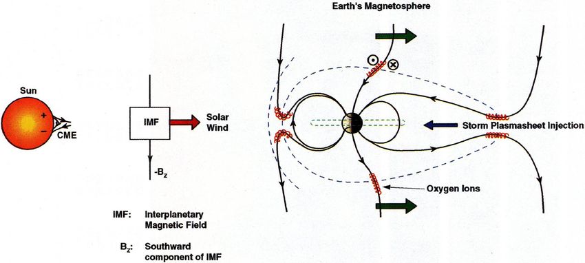
76                                      B. T. Tsurutani et al.: The physics of space weather/solar-terrestrial physics (STP)

of a causal relationship were there in 1859. After Carring-       topic of interplanetary shocks and their acceleration of ener-
ton (1959) published his seminal paper, Hale (1931), New-         getic particles in interplanetary space and also their creating
ton (1943) and others showed that magnetic storms were de-        new radiation belts inside the magnetosphere. Interplanetary
layed by several days from intense solar flares. These types of   shock impingement onto the magnetosphere create dayside
magnetic storms are now known to be caused by either their        auroras and also trigger nightside substorms. Prompt pene-
associated interplanetary coronal mass ejections (ICMEs) or       tration electric fields during magnetic storm main phases will
their upstream sheaths. Details will be discussed later in this   be discussed in terms of the consequences of positive and
review.                                                           negative ionospheric storms, depending on the local time of
   Maunder (1904) showed that geomagnetic activity often          the observation and the phase of the magnetic storm. Two
had a ∼ 27 d recurrence. This periodicity was associated with     relatively new topics, that of supersubstorms (SSSs) and the
some mysteriously unseen (by visible light) feature on the        possibility of precipitating magnetospheric relativistic elec-
Sun. Chree (1905, 1913) showed that these data were statisti-     trons affecting atmospheric weather, will be discussed. A
cally significant, thus inventing the Chree “superposed epoch     glossary will be provided to give definitions of the terms used
analysis”, a scientific data analysis technique which is still    in this review article.
used today. The mysteriously unseen solar features respon-           There have been some recent books and articles that touch
sible for the geomagnetic activity were called “M-regions”        on the many topics of the physics of space weather, though
by Bartels (1934), where the “M” stood for “magnetically          not in the same way that we will attempt to do here. We
active”. It is now known that M regions are coronal holes         recommend for the interested reader “From the Sun: Auro-
(Krieger et al., 1973), solar regions from which solar wind       ras, Magnetic Storms, Solar Flares, Cosmic Rays” by Suess
high-speed streams (HSSs) emanate, causing geomagnetic            and Tsurutani (1998), “Magnetic Storms” by Tsurutani et
activity at the Earth (Sheeley et al., 1976, 1977; Tsurutani      al. (1997a), “Storm-Substorm Relationship” by Sharma et
et al., 1995). The current status of geomagnetic activity as-     al. (2004), “Recurrent Magnetic Storms: Corotating Solar
sociated with HSSs and the future work needed to better un-       Wind Streams” by Tsurutani et al. (2006a), “The Sun and
derstand and to predict the various facets of space weather       Space Weather” by Hanslmeier (2007), “Physics of Space
events will be discussed later.                                   Storms: From the Solar Surface to the Earth” by Koski-
   With the advent of rockets and satellites, the near-Earth      nen (2011), and “Extreme Events in Geospace: Origins, Pre-
interplanetary medium has been probed by magnetic field,          dictability and Consequences” by Buzulukova (2018). Be-
plasma, and energetic particle detectors. The Sun has been        cause space weather is an enormous field/topic, not all facets
viewed at many different wavelengths. The Earth’s auroral         of it have ever been covered in one book. The present au-
regions have recently been viewed by UV imagers, giving a         thors are active researchers in the field and will attempt to in-
global view of auroras including the dayside. The ionosphere      troduce new viewpoints and topics not covered in the above
has been probed by Global Positioning System (GPS) dual-          works.
frequency radio signals, allowing a global map of the iono-
spheric total electron content (TEC) at relatively high spa-      1.2   Organization of the paper
tial and temporal resolution. The purpose of this review arti-
cle will be to give a reasonably thorough review of some of       The concept of magnetic reconnection is introduced first for
the major space weather effects in the magnetosphere, iono-       the non-space plasma reader. Magnetic reconnection is the
sphere and atmosphere and in interplanetary space in order        physical process responsible for transferring solar wind en-
to explain what the solar and interplanetary causes are or are    ergy into the magnetosphere during magnetic storms. We
expected to be. The most useful part of this review will be to    have organized the rest of the paper by discussing space
focus on what future advances in space weather might be in        weather phenomena by solar cycle intervals. However, it
the next 10 to 25 years. In particular, we will mention which     should be mentioned that this is not totally successful since
outstanding problems the Parker Solar Probe, Solar Orbiter,       some phenomena span all parts of the solar cycle.
MMS, Arase, ICON, GOLD, and SWARM data might be                      Solar maximum phenomena such as CMEs, ICMEs, fast
useful in solving.                                                shocks, sheaths, and the forecasting of geomagnetic storms
   Our discussion will first start with phenomena that oc-        associated with the above are covered in Sects. 2.1 to 2.4.
cur most frequently during solar maxima (flares, CMEs and         The space weather phenomena associated with the declin-
ICME-induced magnetic storms). We will explain to the             ing phase of the solar cycle are discussed in Sect. 3. Top-
reader what is meant by an ICME and why we distinguish            ics such as CIRs, CIR storms, HSSs, embedded Alfvén wave
this from a CME. Next, phenomena associated with the de-          trains within HSSs, HILDCAA events, relativistic magneto-
clining phase of the solar cycle will be addressed. These in-     spheric electron acceleration and loss, and electron precipi-
clude corotating interaction regions (CIRs) and HSSs, which       tation and ozone depletion are discussed in Sects. 3.1 to 3.6.
cause high-intensity long-duration continuous AE activity         Although interplanetary shocks are primarily features asso-
(HILDCAA) events and the acceleration and loss of mag-            ciated with fast ICMEs and thus primarily a solar maximum
netospheric relativistic electrons. We will then return to the    phenomenon, shocks can also bound CIRs (∼ 20 % of the

Nonlin. Processes Geophys., 27, 75–119, 2020                                 www.nonlin-processes-geophys.net/27/75/2020/
B. T. Tsurutani et al.: The physics of space weather/solar-terrestrial physics (STP)                                           77

time) at 1 AU during the solar cycle declining phase as well.      nect in the tail. Reconnection leads to strong convection of
Shocks and the high-density plasmas that they create can in-       the plasma sheet into the nightside magnetosphere.
put ram energy into the magnetosphere. Topics such as so-             What is known by theory and verified by observations is
lar cosmic ray particle acceleration, dayside auroras, trigger-    that the stronger the southward component of the IMF and
ing of nightside substorms and the creation of new magne-          the stronger the solar wind velocity convecting the magnetic
tospheric radiation belts are covered in Sects. 4.1 to 4.4. So-    field, the more strongly the solar wind–magnetospheric sys-
lar flares and ionospheric TEC increases are another space         tem is driven (e.g., Gonzalez et al., 1994). Intense IMF Bsouth
weather effect causing direct solar–ionospheric coupling not       in MCs (and sheaths) drives intense magnetic reconnection
involving interplanetary space or the magnetosphere. This is       at the dayside magnetopause and intense reconnection on the
briefly discussed in Sect. 5. Prompt penetration electric fields   nightside. Strong nightside magnetic reconnection leads to
(PPEFs) and ionospheric TEC increases (and decreases) oc-          strong inward convection of the plasma sheet. The stronger
cur during magnetic storms. Although the biggest effects are       the magnetotail reconnection, the stronger the inward con-
observed during ICME magnetic storms (solar maximum),              vection. Via conservation of the first two adiabatic invariants
effects have been noted in CIR magnetic storms as well. This       (Alfvén, 1950), the greater the convection, the greater the en-
is discussed in Sect. 6. The Carrington magnetic storm is          ergization of the radiation belt particles.
the most intense magnetic storm in recorded history. The              As the midnight sector plasma sheet is convected inward to
aurora associated with the storm reached 23◦ from the ge-          lower L, the initially ∼ 100 eV to 1 keV plasma-sheet elec-
omagnetic equator (Kimball, 1960), the lowest in recorded          trons and protons are adiabatically compressed (kinetically
history. Since this event has been used as an example of ex-       energized) so that the perpendicular (to the ambient mag-
treme space weather and events of this type are a problem for      netic field) energy becomes greater than the parallel energy.
U.S. Homeland Security, we felt that there should be a sepa-       This leads to plasma instabilities, wave growth and wave–
rate section on this topic, Sect. 7. We also discuss the possi-    particle interactions (Kennel and Petschek, 1966). The resul-
bility of events even larger than the Carrington storm occur-      tant effect is the “diffuse aurora” caused by the precipitation
ring. In Sect. 8 auroral SSSs are discussed. Why is this topic     of the ∼ 10 to 100 keV electrons and protons into the upper
covered in this paper? It is possible that SSSs which occur        atmosphere/lower ionosphere. At the same time double lay-
within superstorms are the actual causes of the extreme iono-      ers are formed just above the ionosphere, giving rise to ∼ 1
spheric currents, geomagnetically induced currents (GICs),         to 10 keV “monoenergetic” electron acceleration and precip-
that are responsible for potential power grid failures, and        itation in the formation of “discrete auroras” (Carlson et al.,
not the geomagnetic storms themselves. Section 9 gives our         1998).
summary/conclusions for the physics and the possibility of            If the IMF southward component is particularly intense,
forecasting space weather events. Section 10 is a glossary of      this can lead to a magnetic storm with Dst
78                                      B. T. Tsurutani et al.: The physics of space weather/solar-terrestrial physics (STP)

Figure 1. Magnetic reconnection powering geomagnetic storms and substorms. Adapted from Dungey (1961).

2.2   Coronal mass ejections (CMEs), interplanetary
      coronal mass ejections (ICMEs) and magnetic
      storms

What are the solar and interplanetary sources of intense IMFs
that lead to magnetic reconnection at Earth and intense mag-
netic storms? What we know from space age observations is
that these magnetic fields come from parts of a CME, a gi-
ant blob of plasma and magnetic fields which are released
from the Sun associated with solar flares and disappearing
filaments (Tang et al., 1989). Figure 2 shows the emergence
of a CME from behind a solar occulting disk. The time se-
quence starts at the upper left, goes to the right and then to
the bottom left, and ends at the bottom right. The three parts
of a CME are best noted in the image on the bottom left.
There is a bright outer loop most distant from the Sun, fol-
lowed by a “dark region”, and then closest to the Sun is the
solar filament.

2.3   Forecasting magnetic storms and extreme storms
      associated with ICMEs
                                                                   Figure 2. A sequence of images showing the emergence of parts of
We will precede ourselves and state here that for the lim-         a CME coming from the Sun. The time sequence starts at the upper
ited number of cases studied to date, the most geoeffective        left and ends at the lower right. Taken from Illing and Hundhausen
part of the CME is the “dark region”. Interplanetary sci-          (1986).
entists (Burlaga et al., 1981; Choe et al., 1982; Tsurutani
and Gonzalez, 1994) have identified this as the low-plasma
beta region called a magnetic cloud (MC), first identified by      faster than ∼ 700 km s−1 . Only very few have speeds
Burlaga et al. (1981) and Klein and Burlaga (1982) in inter-       >2000 km s−1 , and these come from coronal regions asso-
planetary space by magnetic field and plasma measurements.         ciated with active regions (ARs) (Yashiro et al., 2004).
When there are southward component magnetic fields within              Interplanetary and magnetospheric scientists have devel-
the MC (thought to typically be a giant flux rope), a magnetic     oped the term ICME or interplanetary CME because it is
storm results (Gonzalez and Tsurutani, 1987; Gonzalez et al.,      not currently known (for individual events) how the CME
1994; Tsurutani et al., 1997b; Zhang et al., 2007; Echer et al.,   evolves as it propagates from the Sun to the Earth and be-
2008a).                                                            yond. Leamon et al. (2004), in comparing interplanetary
   It should be noted that fast CMEs and intense MC                MCs to associated solar active regions, found that there was
fields are relatively rare. The SOHO LASCO instrument              little or no relationship, compelling the authors to conclude
has observed >10 000 CMEs, but only ∼ 5 % have speeds              that “MCs are formed during magnetic reconnection and

Nonlin. Processes Geophys., 27, 75–119, 2020                                  www.nonlin-processes-geophys.net/27/75/2020/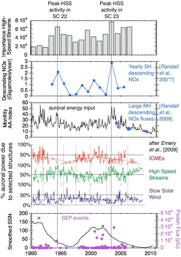
B. T. Tsurutani et al.: The physics of space weather/solar-terrestrial physics (STP)                                                 79

are not simple eruptions of preexisting coronal structures”.
Yurchyshyn et al. (2007) in a similar study found that “for the
majority of interplanetary MCs, the fluxrope axis orientation
changed less than 45◦ going from the Sun to 1 AU”. Palme-
rio et al. (2018) found that “for the majority of cases, the flux
rope tilt angles rotated several tens of degrees (between the
Sun and the Earth) while 35 % changed by more than 90◦ ”.
Three-dimensional MHD simulations have shown that CMEs
can be severely distorted as they interact with different types
of interplanetary structures as they propagate through inter-
planetary space (Odstrcil and Pizzo, 1999a, b). The latter au-
thors have shown that the CME distortion is substantially dif-
ferent when it interacts with the streamer belt (heliospheric
plasma sheet/HPS) than with an HSS. The distortion of the
CME can make the ICME unrecognizable at a distance fur-
ther away from the Sun.
   A more detailed topic not covered in Palmerio et al. (2018)
or in Odstrcil and Pizzo (1999a, b) is the topic of the fate of
the principal features of CMEs as discussed by Illing and
Hundhausen (1986). For example, the bright outer loops are
seldom identified at 1 AU (one rare case was identified by
Tsurutani et al., 1998) and the filaments are typically not
found within the ICME at 1 AU. The first filament detection
at 1 AU was not reported until 1998 (Burlaga et al., 1998).
For more recent observations of filaments at 1 AU, we direct
the reader to Lepri and Zurbuchen (2010). Where have the
bright outer loops and filaments gone to? Have they simply
detached only to impinge onto the magnetosphere at a later
                                                                    Figure 3. An ICME detected at 1 AU just upstream of the Earth.
time, or do they go back into the Sun? Or is it possible that
many CMEs do not have filaments at their bases? Remote
imaging observations from STEREO should be able to an-
swer these questions. New in situ results from Parker Solar            Figure 3 shows a rare case of an ICME at 1 AU where all
Probe, Solar Orbiter and ACE plus ground-based solar ob-            three parts of a CME are detected. The MC is indicated by
servations could perhaps help address the plasma physics of         the shaded region in the figure. The outer loop was identi-
why typical ICMEs do not have attached filaments.                   fied by Tsurutani et al. (1998) and the filament by Burlaga et
   It should be remarked that the high-density solar filaments      al. (1998).
could be extremely geoeffective if they collided with the              From top to bottom are the IMF Bz component (in geocen-
Earth’s magnetosphere (this is covered later in Sect. 3.2.5).       tric solar magnetospheric/GSM coordinates), the field mag-
Is it possible for the MC to rotate so that initially southward     nitude, the solar wind velocity, density, temperature and the
magnetic fields become northward components? Can the MC             He++ /H+ ratio. The bottom panel gives the ground-based
fields be compressed or expanded by interplanetary interac-         Dst index whose amplitude is used as an indicator of the oc-
tions? Can magnetic reconnection be taking place within the         currence of a magnetic storm. Dst becomes negative when
ICME between the solar corona and 1 AU as suggested by              the Earth’s magnetosphere is filled with storm-time energetic
Manchester et al. (2006) and Kozyra et al. (2013)? If so,           ∼ 10–300 keV electrons and ions (Williams et al., 1990).
how often does this occur and can it be predicted? Model-           Dessler and Parker (1959) and Sckopke (1966) have shown
ing and examining the Parker Solar Probe and Solar Orbiter          that the amount of magnetic decrease is linearly related to the
data (for studies on the same ICME) could help us understand        total kinetic energy of the enhanced radiation belt particles.
whether the MCs evolve as they propagate through interplan-         This is because the energetic particles which comprise the
etary space.                                                        storm-time ring current, through gradient drift of the charged
   Of course, the most important goal for space weather is          particles, form a diamagnetic current which decreases the
predicting the southward magnetic fields within the ICME.           Earth’s magnetic field inside the current. We refer the reader
This extremely difficult task is the holy grail of space            to Sugiura (1964) and Davis and Sugiura (1966) for further
weather. It is more important than predicting the time of the       discussions of the Dst index. The Dst index is a 1 h index.
release of a CME, its speed and its direction.                      More recently a 1 min SYM-H index (Iyemori, 1990; Wan-
                                                                    liss and Showalter, 2006) was developed. This is more useful

www.nonlin-processes-geophys.net/27/75/2020/                                     Nonlin. Processes Geophys., 27, 75–119, 2020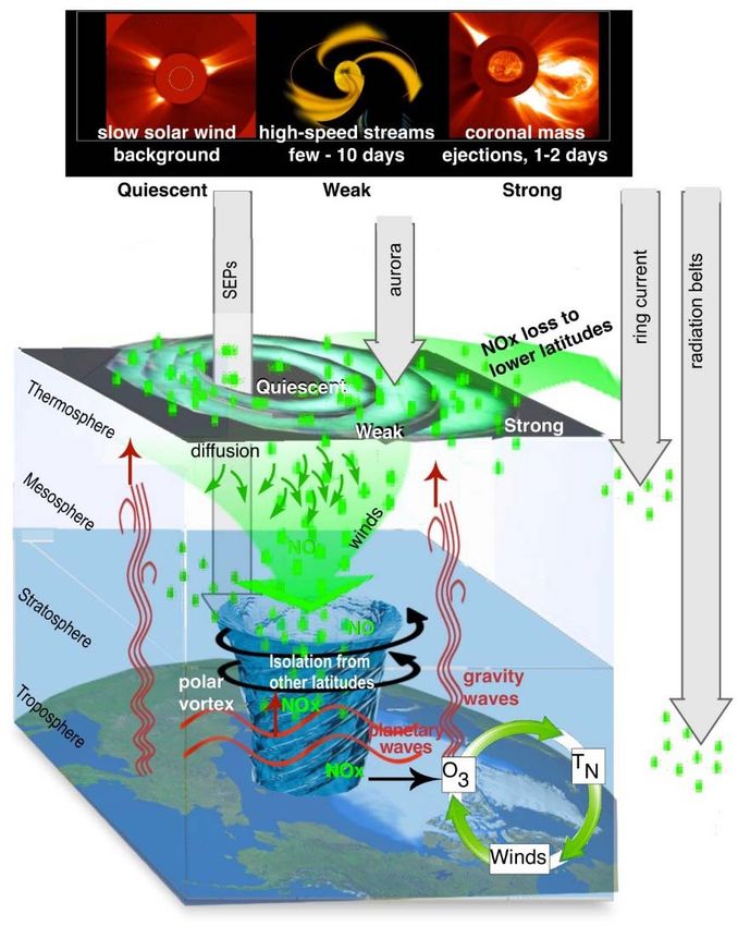
80                                      B. T. Tsurutani et al.: The physics of space weather/solar-terrestrial physics (STP)

for high time resolution studies. Both indices are produced
by the Kyoto Data Center.
    In this example (top panel of Fig. 3) the MC fields start
with a strong southward (Bz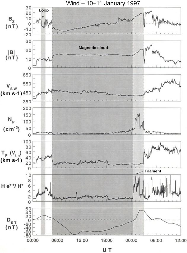
B. T. Tsurutani et al.: The physics of space weather/solar-terrestrial physics (STP)                                                81

                                                                       side system. The magnetic storm Dst index is given at the
                                                                       bottom. Fast forward shocks are denoted by the three vertical
                                                                       red lines on 7 November 2004. There are sudden increases in
                                                                       the velocity, density, temperature and magnetic field magni-
                                                                       tude at all three events. The Rankine–Hugoniot relationships
                                                                       have been applied to the plasma and magnetic field data and
                                                                       the analysis did determine that they are indeed fast shocks.
                                                                          The point of showing this interplanetary event is to indi-
                                                                       cate that each shock pumps up the interplanetary sheath mag-
                                                                       netic field by factors of ∼ 2 to 3. The initial magnetic field
                                                                       magnitude started with a value of ∼ 4 nT, and at the peak
                                                                       value after the three shocks, it reached a value of ∼ 60 nT.
                                                                       This final value was higher than the MC magnetic field,
                                                                       which was ∼ 45 nT. Details concerning the shocks and com-
                                                                       pressions can be found in the original paper for readers who
                                                                       are interested. What is important here is how intense inter-
                                                                       planetary magnetic fields are created. They can come from
Figure 5. An example of three fast forward shocks pumping up           the MCs themselves or the sheaths, as shown here. However,
the interplanetary magnetic field intensity. Taken from Tsurutani et
                                                                       in this case the southward magnetic fields that caused the
al. (2008a).
                                                                       magnetic storm came from the MC and not the sheath.
                                                                          In the above example it is believed that three fast forward
                                                                       shocks were associated with three ICMEs released from the
   Kennel et al. (1985) used MHD simulations to show that              AR. The longitudinal extents of shocks are, however, wider
the plasma densities and magnetic field magnitudes down-               than the MCs, so only one MC was detected in the event. A
stream of shocks are roughly related to the shock magne-               similar situation was found for the August 1972 event dis-
tosonic Mach numbers. This theoretical relationship holds              cussed earlier.
up to a Mach number of ∼ 4. For higher Mach numbers                       It should be noted that a fast reverse wave (here by “re-
MHD predicts that the compression will remain at a factor              verse” we mean that the wave is propagating in the solar di-
of ∼ 4. Since interplanetary shocks detected at 1 AU typi-             rection) was detected during the Fig. 5 event. It is identified
cally have Mach numbers only of 1 to 3 (Tsurutani and Lin,             as the red vertical line on 8 November. In detailed exami-
1985; Echer et al., 2011; Meng et al., 2019), 1 to 3 are the           nation of the Rankine–Hugoniot conservation equations, this
typical shock magnetic field and density compression ratios            wave was found to propagate at a speed below the upstream
detected at 1 AU. One question for future studies is “do the           magnetosonic speed, and thus was a magnetosonic wave and
MHD relationships of magnetic field magnitude and density              not a shock. This reverse wave caused a decrease in the MC
jumps hold for extreme shocks?” If not, there will be impor-           magnetic field (and the southward component) and thus the
tant consequences for extreme space weather.                           start of the recovery phase of the magnetic storm. The reader
   Figure 5 shows a complex interplanetary event that was              should note that fast reverse waves and shocks are also im-
selected by the CAWSES II team to study in detail. The full            portant for geomagnetic activity. A detailed discussion of
information on this event from the Sun to the atmosphere               shock and discontinuity effects on geomagnetic activity can
can be found in the special issue Large Geomagnetic Storms             be found in Tsurutani et al. (2011).
of Solar Cycle 23 (https://agupubs.onlinelibrary.wiley.com/
doi/toc/10.1002/(ISSN)1944-8007.CYCLE231, last access:
                                                                       Forecasting ICME sheath magnetic storms
2008). What is important is that this event was associated
with a solar active region (AR) and the results are quite im-
portant in terms not only of interplanetary disturbance phe-           Determination of the IMF Bz component in the sheaths will
nomena, but also of geomagnetic activity at the Earth.                 be a difficult task. To do this, more effort in understanding
   From top to bottom in Fig. 5 are the solar wind speed,              the slow solar wind plasma, magnetic fields and their vari-
density, and temperature, the IMF Bx , By and Bz com-                  ations will be required. To date, there has been little effort
ponents and the magnetic field magnitude in solar magne-               expended in this area. This is, however, easy for us to hope
tospheric (GSM) coordinates. In this coordinate system, x              for, but in practice it is far more difficult to do. Use of data
points in the direction of the Sun, the y direction is given           from Solar Probe, Solar Orbiter and a 1 AU spacecraft such
by ( × x)/| × x|, where  is the Earth’s south magnetic              as ACE could help in these analyses.
pole (the south magnetic pole is near the north geographic                This problem has recently been emphasized by results
pole), and the z axis, which is in the plane containing both the       from Meng et al. (2019). Meng et al. have shown that su-
Earth–Sun line and the dipole axis, completes the right-hand           perstorms (Dst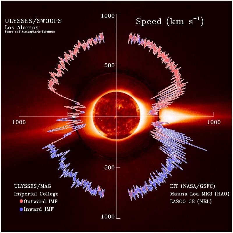
82                                      B. T. Tsurutani et al.: The physics of space weather/solar-terrestrial physics (STP)

                                                                  (top panel). There is a sudden, ∼ tens of seconds’ duration
                                                                  positive increase in Dst which is caused by the sudden in-
                                                                  crease in solar wind ram pressure due to the passage of
                                                                  the sheath high-density jump downstream of the shock. This
                                                                  compresses the magnetosphere, creating the sudden impulse
                                                                  (SI+ : see Joselyn and Tsurutani, 1990) detected everywhere
                                                                  on the ground (Araki et al., 2009). Later, in either the sheath
                                                                  or the MC there may be a southward IMF which causes the
                                                                  magnetic storm. If there is a southward component in the
                                                                  MC, it is usually smoothly varying in intensity and direction.
                                                                  This leads to a smooth monotonically decreasing storm main
                                                                  phase as seen in the Dst index (and illustrated in Figs. 3 and
                                                                  6). The loss of the ring current particles is the cause of the
                                                                  storm recovery phase. The details of storm recovery phase
                                                                  durations and causative mechanisms will be an interesting
                                                                  topic for magnetospheric scientists to study in the near fu-
                                                                  ture. The Arase mission data will be quite useful for these
                                                                  studies.
                                                                     Figure 6b shows the typical profile of a CIR magnetic
                                                                  storm. It is quite different from a sheath-MC magnetic storm
                                                                  profile. There is no SI+ associated with the beginning of the
Figure 6. The magnetic Dst profiles of a CIR magnetic storm (b)   geomagnetic disturbance. This is because CIRs detected at
and an ICME magnetic storm (a). Taken from Tsurutani (2000).      1 AU typically are not led by fast forward shocks (Smith and
                                                                  Wolf, 1976; Tsurutani et al., 1995). The positive increase in
                                                                  Dst is associated with the impact of a high-density region
(1957 to present) are mostly driven by sheath fields or a com-    near the heliospheric current sheet (HCS) (Smith et al., 1978;
bination of sheath plus a following magnetic cloud (MC).          Tsurutani et al., 2006b) called the heliospheric plasma sheet
   Substorms are generated by lower-intensity southward           (HPS; Winterhalter et al., 1994) and/or associated with the
magnetic fields with the process of magnetic reconnection         compressed plasma at the leading edge of the CIR. These are
being the same as above. However, substorm plasma-sheet           slow solar wind plasma densities. The most distinguishing
injections only go in to L ∼ 4, the outer part of the magneto-    feature of the CIR storm main phase is the lack of smooth-
sphere (Soraas et al., 2004). The auroras associated with sub-    ness, in sharp contrast to the MC magnetic storm. This irreg-
storms appear in the “auroral zone”, 60 to 70◦ magnetic lati-     ular Dst storm main phase is caused by large Bz fluctuations
tude (MLAT). Magnetic storms associated with much larger          within the CIR.
IMF Bsouth are detected at subauroral zone latitudes.                CIR magnetic fields have magnitudes of ∼ 20 to 30 nT and
                                                                  typically do not reach the much higher intensities that MC
                                                                  fields typically do. For this reason and also because of the
3     Results: declining phase of the solar cycle                 IMF Bz fluctuations, CIR magnetic storms usually have in-
                                                                  tensities Dst ≥ −100 nT (small or no magnetic storms). Ex-
3.1    Corotating interaction region (CIR) magnetic               treme magnetic storms with Dst < − 250 nT caused by CIRs
       storms                                                     are rare, if they occur at all (none were found in the Meng et
                                                                  al., 2019, study). However, it is clear that compound events
During the declining phase of the solar cycle a different type    involving both CIRs, sheaths ahead of ICMEs and ICMEs
of solar and interplanetary activity dominates the physical       could certainly cause extreme magnetic storm events.
cause of magnetic storms, that of corotating interaction re-         CIR-related magnetic storms occur most frequently during
gions (CIRs). HSSs emanating from coronal holes (CHs) in-         the declining phase of the solar cycle, and ICME magnetic
teract with the slow solar wind and form CIRs at their inter-     storms typically occur near the maximum phase of the solar
action interfaces. The magnetic storms caused by CIRs are         cycle. However, it should be noted that both CIR storms and
quite different from storms caused by ICMEs and/or their          sheath and/or ICME MC magnetic storms can occur during
sheaths. Figure 6 shows the difference in profiles of two dif-    any phase of the solar cycle. We have simply ordered things
ferent types of magnetic storms. The profile of a CIR mag-        by solar cycle so that it will be easier to give the reader the
netic storm is shown at the bottom and that of a shock sheath     general picture of space weather.
ahead of an ICME MC magnetic storm on top.
   The ICME MC magnetic storm Dst profile, discussed
briefly earlier (see Fig. 3), is reasonably easy to identify

Nonlin. Processes Geophys., 27, 75–119, 2020                                 www.nonlin-processes-geophys.net/27/75/2020/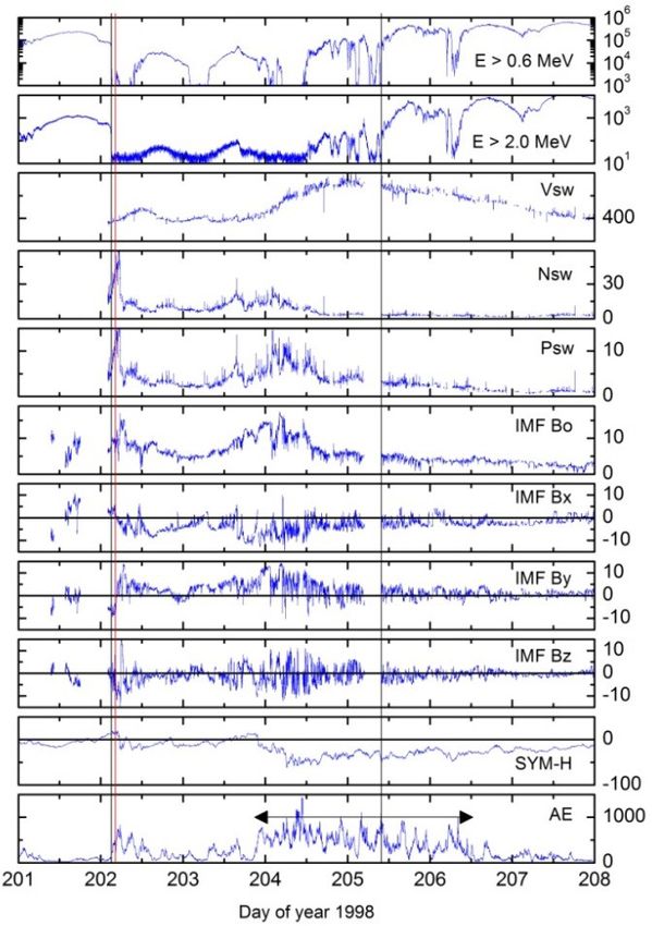
B. T. Tsurutani et al.: The physics of space weather/solar-terrestrial physics (STP)                                                   83

Figure 7. A large coronal hole (the dark region) near the north pole
of the Sun. The figure was taken by the soft X-ray telescope (SXT)
onboard the Yohkoh satellite in 1992.

3.2     Coronal holes, high-speed solar wind streams and               Figure 8. High-speed solar wind streams emanating from coronal
        geomagnetic activity                                           holes in the north and south solar poles. The figure was taken from
                                                                       Phillips et al. (1995) and Tsurutani (2006b).
3.2.1    Coronal holes and high-speed solar wind streams

Figure 7 shows a polar coronal hole at the north pole of the           3.2.2   High-speed solar wind streams and the formation
Sun. This image was taken by the soft X-ray telescope (SXT)                    of CIRs
onboard the Yokoh satellite (http://www.spaceweathercenter.
org/swop/Gallery/Solar_pics/yohkoh_060892.html, last ac-               Figure 9 shows a HSS–slow speed stream interaction dur-
cess: 2002). The dark (low-temperature) region at the pole             ing January 1974. The right portion of the top panel on day
is the coronal hole. Large polar coronal holes occur typically         26 shows a HSS with speeds of 750–800 km s−1 at 1 AU.
in the declining phase of the solar cycle (Bravo and Otaola,           On day 24, the top panel left indicates a solar wind speed
1989; Bravo and Stewart, 1997; Zhang et al., 2005).                    of ∼ 300 km s−1 , or the slow solar wind. The effects of
   Figure 8 gives a “dial plot” of the solar wind speed for            the stream–stream interaction occur on day 25. This is best
the first traversal of the Ulysses spacecraft over the Sun’s           seen in the IMF magnitude panel, seventh from the top. The
poles. The radius from the center of the Sun to the trace in-          stream–stream interaction creates intense magnetic fields of
dicates the solar wind speed. The magnetic field polarity is           ∼ 25 nT. The sixth from top panel is the IMF Bz component
indicated by the color of the trace, red for outward IMFs and          (in GSM coordinates). The Bz is highly fluctuating. Mag-
blue for inward IMFs. A SOHO EIT soft X-ray image of the               netic reconnection between the IMF southward components
Sun is placed at the center of the figure and a High Altitude          and the magnetopause magnetic fields leads to the irregularly
Observatory Mauna Loa coronagraph image shows the inner                shaped storm main phase shown in the bottom (Dst ) panel.
corona at that time. The outer corona is an image taken by                To be able to forecast a CIR magnetic storm, one would
the SOHO C2 coronagraph.                                               have to first understand the sources of the IMF Bz fields. For
   Two large polar coronal holes are detected at the Sun, one          example, are they compressed upstream Alfvén waves (Tsu-
at the north pole and the other at the south pole. It is noted         rutani et al., 1995, 2006c)? Or could they be waves generated
that HSSs of ∼ 750 to 800 km s−1 are detected at Ulysses               by the shock interaction with upstream waves in the slow so-
when over the polar coronal hole regions. When Ulysses was             lar wind? That would be only the first step for forecasting,
near the solar equatorial region where helmet streamers are            of course. Then with knowledge of the properties of the slow
present, the solar wind speeds are of the slow solar wind va-          speed stream, the details of the wave compression/interaction
riety, Vsw ∼ 400 km s−1 . The reader should note that it took          would then have to be calculated/modeled.
years for Ulysses to make this polar orbit, while the solar and           Another approach would be to determine whether there
coronal images were taken at one point in time. However, this          is an underlying southward component of the IMF within
composite figure is useful to illustrate the main points about         the CIR. This would most likely be caused by the geome-
the origins of HSSs.                                                   try of the HSS–slow speed stream interaction and may be

www.nonlin-processes-geophys.net/27/75/2020/                                        Nonlin. Processes Geophys., 27, 75–119, 2020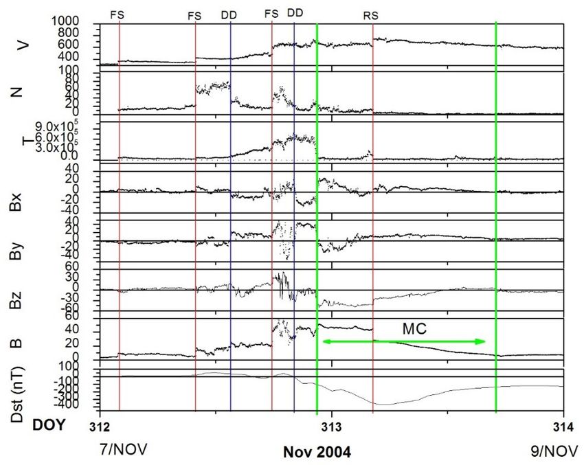
84                                          B. T. Tsurutani et al.: The physics of space weather/solar-terrestrial physics (STP)

                                                                         Figure 10. A high-intensity, long-duration continuous AE ac-
Figure 9. A high-speed solar wind stream–slow solar wind interac-        tivity (HILDCAA) event during 1974. Taken from Tsurutani et
tion and the formation of a CIR during January 1974. The format is       al. (2006c).
the same as in Fig. 4 except that the AE index is given in the next to
bottom panel. The figure is taken from Tsurutani et al. (2006b).

                                                                            The interplanetary data were taken from the IMP-8 space-
predictable from MHD modeling. If this is correct, then the              craft, an Earth-orbiting satellite that was located upstream of
sheath fields can be modelled by a slowly varying field with             the magnetosphere in the solar wind at this time. The location
highly fluctuating fields superposed on top of it. In (rare)             was inside 40 Re, where an Re is an Earth radius. The mag-
cases of radial alignment, Solar Probe closest to the Sun                netic Bz fluctuations have been shown to be Alfvén waves
could characterize sheath fields. The evolution of those fields          which are of large nonlinear amplitudes in HSSs (Belcher
would be detected by Solar Orbiter. Simulation of further                and Davis, 1971; Tsurutani and Gonzalez, 1987; Tsurutani
evolution could be applied and predictions of the fields at              et al., 2018b). What is apparent from this figure is that every
1 AU could be tested by ACE data. If there are waves gener-              time the IMF Bz is negative (southward), there is an AE in-
ated by the shock, then the above scenario would not work                crease and a Dst decrease. This has been interpreted as being
as well as expected, or at least would be more complicated to            due to magnetic reconnection between the southward compo-
apply in a useful manner.                                                nents of the Alfvén waves and the Earth’s magnetopause. The
                                                                         AE is enhanced by the same magnetic reconnection process
3.2.3   High-speed solar wind streams, Alfvén waves and                  that occurs during substorms, and a small parcel of plasma-
        HILDCAAs                                                         sheet plasma is injected into the nightside magnetosphere,
                                                                         causing the Dst index to decrease slightly. It is noted that
The schematic in Fig. 6 showed a long “recovery phase” that              there are many southward IMF Bz dips in this 4-day interval
trails the CIR magnetic storm main phase (see Tsurutani and              of data shown in Fig. 10. There are also many corresponding
Gonzalez, 1987). However, we now know that the storm was                 AE increases and Dst decreases. Thus, the interpretation of
not “recovering” as in the case of an MC magnetic storm                  the constant/average Dst value of ∼ −25 nT for 4 days is that
recovery but that something else was occurring. This “recov-             continuous plasma injection and decay are occurring. This is
ery” can last from days to weeks. Thus, processes of charge              clearly not a “recovery phase” where the ring current parti-
exchange, Coulomb collisions, etc., for ring current particle            cles are simply lost; it only appears as a recovery from the
losses are not tenable to explain such long “recoveries”.                Dst trace. Soraas et al. (2004) have shown that particles are
   Figure 10 shows the interplanetary cause of this extended             injected during these events, but only to L values of 4 and
geomagnetic activity. It occurs primarily during HSSs inde-              greater (the L = 4 magnetic field line is the dipole magnetic
pendent of whether a CIR magnetic storm occurred prior to it             field that crosses the magnetic equator a distance of 4 Earth
or not (Tsurutani and Gonzalez, 1987; Tsurutani et al., 1995,            radii from the center of the Earth). These are shallow injec-
2006b; Kozyra et al., 2006b; Turner et al., 2006; Hajra et al.,          tions, as suggested above.
2013, 2014a, b, c, 2017). From top to bottom are the solar                  These geomagnetic activity events have been named high-
wind speed, the IMF magnitude, the IMF Bz component (in                  intensity, long-duration continuous AE events or HILDCAAs
GSM coordinates) and the auroral electrojet (AE) index. The              (Tsurutani and Gonzalez, 1987). This name is simply a de-
bottom panel is the Dst index.                                           scription of the events without an interpretation. In 2004
                                                                         when a detailed examination using polar EUV auroral imag-

Nonlin. Processes Geophys., 27, 75–119, 2020                                        www.nonlin-processes-geophys.net/27/75/2020/
B. T. Tsurutani et al.: The physics of space weather/solar-terrestrial physics (STP) 85
ing was applied, it was found that many phenomena be-
sides simple isolated substorms occurred (Guarnieri, 2006;
Guarnieri et al., 2006). Although substorms occur during
HILDCAA events, there are AE increases (injection events?)
that are not well correlated with substorm onsets (Tsurutani
et al., 2004b). The full extent of HILCAAs is not well un-
derstood (see also Souza et al., 2016; Marques de Souza et
al., 2018; Mendes et al., 2017). By using IMAGE auroral
observations and geomagnetic indices to identify convection
events which are not classical Akasofu (1964) substorms, the
fields and particle data from SWARM, MMS and Arase could
be used to characterize the physics properties of these “con-
vection” events.
There is also the question of the origin of the interplane-
tary Alfvén waves. Do they originate at the Sun caused by
supergranular circulation or is that mechanism untenable, as
argued by Hollweg (2006)? Could the waves be generated lo-
cally between the Sun and Earth, as speculated by Matteini et
al. (2006, 2007) and Hellinger and Travnicek (2008)? Parker
Solar Probe could identify Alfvén waves within high-speed
streams and Solar Orbiter (when radially aligned) could de-
termine the wave evolution.
The original requirement for identifying a HILCAA event
was quite strict. The event had to occur outside of a magnetic
storm main phase (Dst was required to be > − 50 nT: Gon-
zalez et al., 1994), the peak AE intensity had to be greater Figure 11. The relationship between HILDCAAs and relativistic
than 1000 nT (high-intensity), the event had to last longer electron acceleration. The figure is taken from Hajra et al. (2015a).
than 2 d (long-duration), and there could not be any dips in
AE less than 200 nT for longer than 2 h (continuous). Clearly
there are events with the same interplanetary causes and ge- The figure shows that the flux enhancement of
omagnetic effects as for the strict definition. However, the E>0.6 MeV electrons is statistically delayed by ∼ 1.0 d
strict definition is useful for further studies using different from the onset of the HILDCAAs. The E>4.0 MeV
data sets. electrons are statistically delayed by ∼ 2.0 d from the
HILDCAA onset. It is thus possible that HILCAAs may
3.2.4 HILDCAAs and the acceleration of relativistic be used to forecast relativistic electron flux enhancements
magnetospheric electrons in the magnetosphere (see Hajra et al., 2015b; Tsurutani
et al., 2016a; Hajra and Tsurutani, 2018a; Guarnieri et al.,
One of the consequences of HSSs and HILDCAAs is the ac- 2018). This however has not been done yet and could be
celeration of relativistic (∼ MeV) electrons. These energetic implemented by scientists today.
particles can damage orbiting satellite electronic components The physics for electron acceleration to relativistic
(Wrenn, 1995) and thus are known as “killer electrons”. Fig- (∼ MeV) energies has been well developed by magneto-
ure 11 shows the relationship between the onset of HILCAA spheric scientists. Two competing acceleration mechanisms
events (vertical line) and relativistic electron fluxes. From have been developed. In one mechanism, with each injection
top to bottom are the E>0.6 MeV, the E>2.0 MeV and the of plasma-sheet particles on the nightside magnetosphere,
E>4.0 MeV electron fluxes detected by the GOES-8 and the anisotropic ∼ 10 to 100 keV electrons generate electro-
GOES-12 satellites located at L = 6.6. This figure is a super- magnetic whistler mode chorus waves (Tsurutani and Smith,
posed epoch analysis (Chree, 1913), the result of 35 HILD- 1974; Meredith et al., 2002) by the loss cone/temperature
CAA events in solar cycle 23, from 1995 to 2008, which are anisotropy instability (Brice, 1964; Kennel and Petschek,
not preceded by magnetic storms. The exclusion of magnetic 1966; Tsurutani et al., 1979; Tsurutani and Lakhina, 1997).
storms was done to avoid contamination by storm-time par- The chorus then interacts with the ∼ 100 keV injected elec-
ticle acceleration (by intense convection/compression). The trons to energize them to ∼ 0.6 MeV energies (Inan et al.,
zero-epoch time (vertical line) corresponds to the HILDCAA 1978; Horne and Thorne, 1998; Thorne et al., 2005, 2013;
onset time. Here the “strict” definition of HILDCAAs was Summers et al., 2007; Tsurutani et al., 2010; Reeves et al.,
used to define the onset times. 2013; Boyd et al., 2014). The lower-frequency part of the
chorus in turn interacts with the ∼ 0.6 MeV electrons to
www.nonlin-processes-geophys.net/27/75/2020/ Nonlin. Processes Geophys., 27, 75–119, 202086 B. T. Tsurutani et al.: The physics of space weather/solar-terrestrial physics (STP)
accelerate them to ∼ 2.0 MeV energies. This bootstrapping
mechanism has been suggested by several authors (Baker et
al., 1979, 1998; Li et al., 2005; Turner and Li, 2008; Boyd et
al., 2014, 2016; Reeves et al., 2016) and has been confirmed
by Hajra et al. (2015a) during HILDCAA events.
An alternative scenario is that relativistic electrons are cre-
ated through particle radial diffusion driven by micropulsa-
tions (Elkington et al., 1999, 2003; Hudson et al., 1999; Li et
al., 2001; O’Brien et al., 2001; Mann et al., 2004; Miyoshi et
al., 2004). However, the same general scenario would hold as
for chorus acceleration. The substorms and convection events
within HILDCAAs would be the sources of the micropulsa-
tions and the micropulsations would last from days to weeks
in duration. Bootstrapping of energy would still take place.
An important question for researchers to ask is “How high
can the relativistic magnetospheric electron energy get?”. If
there are two HSSs, one from the South Pole and another
from the North Pole so that Earth’s magnetosphere is bathed
in HSSs for years, as happened during 1973–1975 (Shee-
ley et al., 1976, 1977; Gosling et al., 1976; Tsurutani et
al., 1995), will the energies go above ∼ 10 MeV? What will
physically limit the energy range? This answer is important
for keeping Earth-orbiting satellites safe during such events.
3.2.5 Solar wind ram pressure pulses and the loss of
relativistic electrons
Figure 12 shows a relativistic electron decrease (RED)
event occurring during 1998. From top to bottom are the
E>0.6 MeV electron fluxes, the E>2.0 MeV electron fluxes, Figure 12. A relativistic electron decrease (RED) event and later
the solar wind speed, density and ram pressure, and the IMF acceleration. Taken from Tsurutani et al. (2016b).
magnitude and Bx , By and Bz components in the GSM co-
ordinate system. The bottom two panels are the 1 min SYM-
H index (a high time resolution Dst index) and the AE in- ond possible mechanism is electron pitch angle scattering by
dex. The relativistic electron measurements were taken at electromagnetic ion cyclotron (EMIC) waves. We think that
L = 6.6. this second possibility is more intriguing and has far more
At the beginning of day 202, a vertical black line indi- interesting consequences, if correct. One might ask where
cates the onset of a high-density HPS crossing (Winterhalter the EMIC waves come from and why pitch angle scatter-
et al., 1994) that is identified in the fourth panel from the ing is particularly important. It has been shown by Remya et
top. The HPS is by definition located adjacent to the HCS al. (2015) that when the magnetosphere is compressed, both
(Smith et al., 1978). The HCS is noted by the reversal in electromagnetic chorus (electron) waves (Thorne et al., 1974;
the signs of the IMF Bx and By components (seventh and Tsurutani and Smith, 1974; Meredith et al., 2002) and EMIC
eighth panels from the top). The onset of the HPS is followed (ion) waves (Cornwall, 1965; Kennel and Petschek, 1966;
within 1 h by the vertical red line, the sudden disappearance Olsen and Lee, 1983; Anderson and Hamilton, 1993; En-
of the E>0.6 MeV (first panel) and E>2.0 MeV (second gebretson et al., 2002; Halford et al., 2010; Usanova, 2012;
panel) relativistic electron fluxes. Tsurutani et al. (2016b) Saikin, 2016) are generated. The compression of the mag-
have shown that for eight relativistic electron flux disappear- netosphere causes betatron acceleration of remnant ∼ 10 to
ance events during solar cycle 23 all of the disappearances 100 keV electrons and protons, and thus plasma instabilities
were associated with HPS impingements onto the magneto- associated with both particle populations occur. What is par-
sphere. ticularly important is that the EMIC waves are coherent (Re-
Where have the relativistic electrons gone? There are two mya et al., 2015), leading to extremely rapid pitch angle scat-
primary possibilities. One is that the energetic electrons have tering of ∼ 1 MeV electrons by the waves. The scattering rate
gradient drifted out of the magnetosphere through the day- has been shown to be 3 orders of magnitude faster than that
side magnetopause, a feature that has been called “magne- with incoherent waves (Tsurutani et al., 2016b).
topause shadowing” by West et al. (1972). However, a sec-
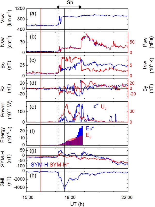
Nonlin. Processes Geophys., 27, 75–119, 2020 www.nonlin-processes-geophys.net/27/75/2020/B. T. Tsurutani et al.: The physics of space weather/solar-terrestrial physics (STP) 87 Another possible loss mechanism is associated with pos- possible triggers of high-atmospheric vorticity winds. Quan- sible generation of PC waves by the HPS impingement fol- titative estimates of potential energy deposition at different lowed by radial diffusion of the relativistic electrons. Wygant atmospheric altitudes were provided in the original paper. et al. (1998) and Halford et al. (2015) have mentioned that It is noted that the energy deposition should occur in a lim- larger loss cone sizes at lower L could be a source of loss to ited spatial region of the globe (just inside the auroral zone the ionosphere. Rae et al. (2018) have shown that superposi- and a small region of the dayside atmosphere), which is more tion of compressional PC waves and the conservation of the geoeffective than either cosmic ray energy or solar flare par- first two adiabatic invariants could enhance particle losses. ticle deposition. The fact that it is relativistic electron precip- However, one should mention that there are no observations itation gives an additional advantage that substantial energy of PC wave generation during HPS impingements, and this is deposited at quite low altitudes. needs to be tested. It is also uncertain how rapidly the rela- Advances to this problem can be made in a number of dif- tivistic electrons would be lost by the above processes. It has ferent ways. Simultaneous ground-detected EMIC waves, γ - been shown that the total loss of L>6.6 relativistic electrons rays and atmospheric heating/cooling could be sought. Cor- occurs in ∼ 1 h (Tsurutani et al., 2016b). relation with such events with solar wind pressure pulses like Why can the loss of relativistic electrons to the atmosphere the HPSs or interplanetary shocks (see Hajra and Tsurutani, be important? Figure 13 shows the results of the GEometry 2018b) would advance our knowledge of the details of such ANd Tracking 4 (GEANT4) code developed by the European events. Organization for Nuclear Research (Agostinelli et al., 2003) Maliniemi, Asikainen and Mursula (2014) studied the applied to the relativistic electron disappearance problem. Earth’s winter surface temperatures and the North Atlantic The GEANT4 code takes into account Rayleigh scattering, Oscillation (NAO) during all 4 phases of the solar cycle us- Compton scattering, photon absorption, γ -ray pair produc- ing 13 solar cycles of data (1869–2009). The authors found tion, multiple scattering, ionization, bremsstrahlung for elec- that the clearest pattern for temperature anomalies is not dur- trons and positrons and annihilation of positrons (positron ing sunspot maximum or minimum but during the declin- formation is not germane for these “low energy” relativistic ing phase when the temperature pattern closely resembles particles, but the code includes it anyway). A standard atmo- that found during positive NAO. This feature could be due sphere was used. to the energetic 10–100 keV electron precipitation discussed Figure 13 shows the GEANT4 Monte Carlo results for the earlier. electron shower for E>0.6 MeV electrons on the left and Atmospheric heating events known as sudden strato- for E>2.0 MeV electrons on the right. Two important fea- spheric warmings (SSWs) (Scherhag, 1960; Harada et al., tures should be noted. First the bulk of energy deposition (the 2010) occur at subauroral latitudes by unknown causes. They red areas) descends to ∼ 60 km for the E>0.6 MeV electron are known to be related to atmospheric wind system changes, simulation and to ∼ 50 km for the E>2.0 MeV electron sim- perhaps the same phenomenon as the Wilcox et al. (1973) ulation. This portion of the energy from the incident elec- effect. Atmospheric scientists generally assume that SSWs trons is due to direct ionization and particle energy cascad- are created by gravity waves propagating from the lower at- ing. However, there is a second region which might be ex- mosphere upward, but so far no one-to-one correlated case tremely important, that is, the blue-green area that goes down has been found. Thus, it would be quite interesting to see to ∼ 20 km for the E>0.6 MeV simulation and ∼ 16 km for whether space weather can have a major impact on atmo- the E>2.0 MeV simulation. There are also “hits” seen on the spheric weather. The connection between these two disci- ground. This lower-altitude energy deposition is due to the plines could be quite interesting for the next generation of relativistic electrons interacting with atmospheric atomic and space weather scientists. molecular nuclei creating bremsstrahlung X-rays and γ -rays. X-rays and γ -rays have very large mean free paths and thus 3.2.6 Energetic particle precipitation and ozone can freely propagate through the dense atmosphere without depletion interactions. They propagate to much lower altitudes where they interact and continue the energy cascading process fur- Figure 14 shows two solar cycles of data, SC22 and SC23. ther. From top to bottom are the “importance” of high-speed The reason why this process may be quite an important streams, the descending NOx , the monthly AA index, and space weather topic is that it might relate to atmospheric the percent auroral power due to three types of solar wind weather as well. Wilcox et al. (1973) discovered a correlation phenomena (ICMEs, HSSs and slow solar wind), and the between interplanetary HCS crossings and high-atmospheric bottom panel solid line trace is the sunspot number (SSN). vorticity winds at 300 mb altitude. Over the years a number Also shown in the bottom panel is the solar energetic particle of different explanations for the physics of the trigger have (SEP) flux. been offered (Tinsley and Deen, 1991; Lam et al., 2013). There are two vertical dashed lines. They correspond to the Tsurutani et al. (2016b) presented the above relativistic elec- peaks in HSS activity for SC22 and SC23 (top panel), peaks tron precipitation scenario (instead of HCS crossings) for the in auroral energy input (third panel from the top), and peaks www.nonlin-processes-geophys.net/27/75/2020/ Nonlin. Processes Geophys., 27, 75–119, 2020
88                                         B. T. Tsurutani et al.: The physics of space weather/solar-terrestrial physics (STP)

Figure 13. The GEANT4 code run results for the precipitation of E>0.6 MeV electrons (left panel) and E>2.0 MeV electrons (right panel).
The vertical scale is altitude above the ground and the horizontal scale is energy deposition. The color scheme (legend on the right) gives the
number of counts. Taken from Tsurutani et al. (2016b).

                                                                          in the yearly descending NOx (second panel from the top).
                                                                          It is noted that all three peaks are aligned in time. The bot-
                                                                          tom panel shows that both dashed vertical lines correspond
                                                                          to times in the descending phase of the solar cycle.
                                                                             Figure 15 shows the Kozyra et al. (2019) scenario for
                                                                          ozone destruction over the polar cap. The top of the figure
                                                                          shows the various types of solar wind (and associated ener-
                                                                          getic particles) that can affect atmospheric ozone. The quiet
                                                                          solar wind will lead to quiescence. HSSs lasting a few to 10
                                                                          days have weak effects, and ICMEs (and of course shock ac-
                                                                          celeration of energy particles) can have much stronger ef-
                                                                          fects.
                                                                             Energetic particles from different sources will precipitate
                                                                          in different regions of the ionosphere. The energetic particles
                                                                          associated with interplanetary CME shock acceleration will
                                                                          be deposited in the polar regions of both the northern and
                                                                          southern ionospheres. If the particles are energetic enough
                                                                          with sufficient gyroradii, they can reach latitudes as low as
                                                                          ∼ 50◦ magnetic latitude. Precipitating substorm/HILDCAA
                                                                          ∼ 10–100 keV magnetospheric charged particles will deposit
                                                                          their energy on closed auroral zone (∼ 60 to 70◦ ) magnetic
                                                                          field lines.
                                                                             The energetic particles entering the atmosphere lose a por-
                                                                          tion of their energy in the dissociation of N2 into N + N. The
                                                                          nitrogen atoms will attach to oxygen atoms to form NOx .
                                                                          Auroral HILDCAA ∼ 10–100 kev energy particles will only
                                                                          penetrate to depths of ∼ 75 km above the surface of the Earth.
                                                                          Solar energetic particles with greater kinetic energies can
                                                                          penetrate lower into the atmosphere to ∼ 50 to 60 km. If there
                                                                          is a polar vortex, this vortex can “entrain” the NOx molecules
                                                                          and atmospheric diffusion can bring them down to lower al-
Figure 14. The dashed vertical lines show the peaks in solar wind
                                                                          titudes over months in time duration. The NOx can act as a
high-speed streams during SC 22 and SC 23. These are coincident
with the peaks in auroral energy input and the peaks in yearly NOx
                                                                          catalyst in the destruction of ozone.
descent. The authors thank Janet Kozyra for providing this unpub-            One interesting consequence of extreme ICME shocks is
lished figure.                                                            that one would expect extreme Mach numbers to lead to both
                                                                          extreme SEP fluences and also extremely high energies. The
                                                                          former will lead to greater production of NOx int the po-
                                                                          lar regions and the latter to deeper penetration and thus less

Nonlin. Processes Geophys., 27, 75–119, 2020                                          www.nonlin-processes-geophys.net/27/75/2020/
You can also read