Using Machine Learning to Detect if Two Products Are the Same - Bc. Jung Peter A master thesis from
←
→
Page content transcription
If your browser does not render page correctly, please read the page content below
Using Machine Learning to Detect if
    Two Products Are the Same

                   A master thesis from

                 Bc. Jung Peter

             Faculty of Electrical Engineering
           Czech Technical University in Prague
          Open Informatics, Artificial intelligence
                     Czech Republic
                           2020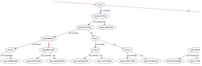
MASTER‘S THESIS ASSIGNMENT

I. Personal and study details

  Student's name:             Jung Peter                                                 Personal ID number:           486798
  Faculty / Institute:        Faculty of Electrical Engineering
  Department / Institute:           Department of Computer Science
  Study program:              Open Informatics
  Specialisation:             Artificial Intelligence

II. Master’s thesis details
  Master’s thesis title in English:
   Using Machine Learning to Detect if Two Products Are the Same

  Master’s thesis title in Czech:
   Využití strojového učení pro detekování, kdy jsou dva produkty stejné

  Guidelines:
   The main goal of this work is to design a prototype of a system for
   predicting when two products (e.g. mobile phones, vacuum cleaners etc.)
   are the same product based on their textual description. The main
   research question is to evaluate feasibility of using character-level and
   word-level word embeddings for this task.
   1. Design a system for predicting when textual descriptions of two
   products refer to the same product. Use insights from [2].
   2. Empirically evaluate feasibility of models based on word embeddings
   for this problem.
   3. Compare performance of character-level (e.g. [4]) and word-level
   word embeddings (e.g. [5]) for this task empirically. Discuss the
   results.

  Bibliography / sources:
   [1] Goodfellow, I., Bengio, Y., & Courville, A. (2016). Deep learning. MIT press.
   [2] More, A. (2017x). Product Matching in eCommerce using deep learning.
   Available online: https://medium.com/walmartlabs/product-matching-in-
   ecommerce-4f19b6aebaca
   [3] Mikolov, T., Sutskever, I., Chen, K., Corrado, G. S., & Dean, J. (2013).
   Distributed representations of words and phrases and their compositionality. In
   Advances in neural information processing systems (pp. 3111-3119).
   [4] Kim, Y., Jernite, Y., Sontag, D., & Rush, A. M. (2016, March). Character-
   aware neural language models. In Thirtieth AAAI Conference on Artificial
   Intelligence.

  Name and workplace of master’s thesis supervisor:
   Ing. Ondřej Kuželka, Ph.D.,            Intelligent Data Analysis, FEE

  Name and workplace of second master’s thesis supervisor or consultant:

   Date of master’s thesis assignment: 04.02.2020                       Deadline for master's thesis submission: 22.05.2020

   Assignment valid until: 30.09.2021

 ___________________________                   ___________________________                  ___________________________
       Ing. Ondřej Kuželka, Ph.D.                       Head of department’s signature             prof. Mgr. Petr Páta, Ph.D.
           Supervisor’s signature                                                                         Dean’s signature

CVUT-CZ-ZDP-2015.1                                                                         © ČVUT v Praze, Design: ČVUT v Praze, VIC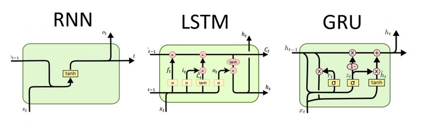
III. Assignment receipt
   The student acknowledges that the master’s thesis is an individual work. The student must produce his thesis without the assistance of others,
   with the exception of provided consultations. Within the master’s thesis, the author must state the names of consultants and include a list of references.

                             .
                        Date of assignment receipt                                                        Student’s signature

CVUT-CZ-ZDP-2015.1                                                                                          © ČVUT v Praze, Design: ČVUT v Praze, VIC
AFFIDAVIT

   I declare that I am the sole author of this diploma thesis on the "Using machine learning to
detect if two products are the same" using the literature and sources mentioned, and with my
supervisor’s great help.

                                                                       Date, city and signature

                                              3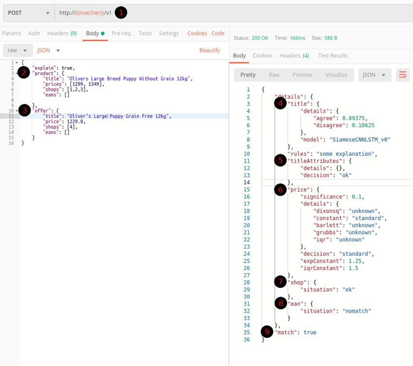
THANKS

   I would like to thank my supervisor, for accepting the idea of this work in the very beginning
and his later professional guidance in terms of machine learning and academic writing.

Not smaller thank also belong to my professors during the last two years, who taught me arti-
ficial intelligence in general.

I also have to mention my work colleagues, for giving me access to the company databases, guiding
me about their usage and computational power of their servers.

                                               4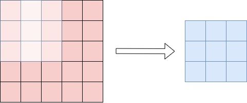
Contents
1 ANNOTATION                                                                                                                            8
  1.1 ENGLISH . . . . . . . . . . . . . . . . . . . . . . . . . . . . . . . . . . . . . . . . .                                         8
  1.2 SLOVAK . . . . . . . . . . . . . . . . . . . . . . . . . . . . . . . . . . . . . . . . .                                          8

2 INTRODUCTION                                                                                                                         9

3 BACKGROUND                                                                                                                            9
  3.1 EMBEDDING . . . . . . . . . . . . . . . . . . . .        .   .   .   .   .   .   .   .   .   .   .   .   .   .   .   .   .   .    9
      3.1.1 WORD-LEVEL . . . . . . . . . . . . . . . .         .   .   .   .   .   .   .   .   .   .   .   .   .   .   .   .   .   .    9
      3.1.2 CHARACTER AND SUB-WORD LEVEL                       .   .   .   .   .   .   .   .   .   .   .   .   .   .   .   .   .   .   10
      3.1.3 DIMENSIONS . . . . . . . . . . . . . . . .         .   .   .   .   .   .   .   .   .   .   .   .   .   .   .   .   .   .   10
  3.2 NEURAL NETWORKS . . . . . . . . . . . . . . .            .   .   .   .   .   .   .   .   .   .   .   .   .   .   .   .   .   .   10
  3.3 CONVOLUTIONAL NEURAL NETWORKS . . .                      .   .   .   .   .   .   .   .   .   .   .   .   .   .   .   .   .   .   10
  3.4 RECURRENT NEURAL NETWORKS . . . . . .                    .   .   .   .   .   .   .   .   .   .   .   .   .   .   .   .   .   .   11
  3.5 SIAMESE NEURAL NETWORKS . . . . . . . . .                .   .   .   .   .   .   .   .   .   .   .   .   .   .   .   .   .   .   11
  3.6 GRADIENT BOOSTING TECHNIQUES . . . . .                   .   .   .   .   .   .   .   .   .   .   .   .   .   .   .   .   .   .   12

4 PROBLEM DESCRIPTION                                                                                                                  12
  4.1 PROBLEM STATEMENT . . . . . . . . . . . . . . . . . . . . . . . . . . . . . . .                                                  12
  4.2 PREVIOUS WORK . . . . . . . . . . . . . . . . . . . . . . . . . . . . . . . . . . .                                              13

5 IN ADDITION TO MACHINE LEARNING                                                             13
  5.1 FINDING PRODUCT CANDIDATES FOR INCOMING OFFERS . . . . . . . . . 13
  5.2 PRICE OUTLIERS . . . . . . . . . . . . . . . . . . . . . . . . . . . . . . . . . . . 14
      5.2.1 GRUBBS’S TEST . . . . . . . . . . . . . . . . . . . . . . . . . . . . . . . . 14
      5.2.2 BARTLETT’S TEST . . . . . . . . . . . . . . . . . . . . . . . . . . . . . . 15
      5.2.3 INTERQUARTILE RANGES . . . . . . . . . . . . . . . . . . . . . . . . . . 15
      5.2.4 DIXON’S Q TEST . . . . . . . . . . . . . . . . . . . . . . . . . . . . . . . . 15
      5.2.5 RATIO THRESHOLD . . . . . . . . . . . . . . . . . . . . . . . . . . . . . . 16
      5.2.6 TESTS . . . . . . . . . . . . . . . . . . . . . . . . . . . . . . . . . . . . . . 16
  5.3 ATTRIBUTES EXTRACTED FROM TITLE . . . . . . . . . . . . . . . . . . . . . 16
      5.3.1 FIRST VERSION OF ATTRIBUTE CHECKING, TOKENIZED EXACT
            MATCH . . . . . . . . . . . . . . . . . . . . . . . . . . . . . . . . . . . . . . 16
      5.3.2 SECOND VERSION OF ATTRIBUTE CHECKING, DAMERAU–LEVENSHTEIN
            VARIANCES WITH THRESHOLD . . . . . . . . . . . . . . . . . . . . . . 17
  5.4 EUROPEAN ARTICLE NUMBERS . . . . . . . . . . . . . . . . . . . . . . . . . . 17
  5.5 PROPOSED API . . . . . . . . . . . . . . . . . . . . . . . . . . . . . . . . . . . . . 17

6 DEEP LEARNING MODEL                                                                                                                  19
  6.1 OBTAINING DATASET FOR TRAINING AND EVALUATION                                            .   .   .   .   .   .   .   .   .   .   19
  6.2 PRODUCT AND OFFERS DOWNLOADING IN GO LANG . .                                            .   .   .   .   .   .   .   .   .   .   19
  6.3 TOKENIZATION . . . . . . . . . . . . . . . . . . . . . . . . . .                         .   .   .   .   .   .   .   .   .   .   20
  6.4 GENERATING PAIRS OF TITLES . . . . . . . . . . . . . . . .                               .   .   .   .   .   .   .   .   .   .   20
      6.4.1 RANDOM MERGE - POSITIVE PAIR . . . . . . . . . .                                   .   .   .   .   .   .   .   .   .   .   21
      6.4.2 SHUFFLE - POSITIVE PAIR . . . . . . . . . . . . . . .                              .   .   .   .   .   .   .   .   .   .   21
      6.4.3 JOIN TOKENS - POSITIVE PAIR . . . . . . . . . . . .                                .   .   .   .   .   .   .   .   .   .   21
      6.4.4 DROP OR SWITCH CHARACTERS - POSITIVE PAIR                                          .   .   .   .   .   .   .   .   .   .   21
      6.4.5 DROP OR DUPLICATE TOKEN - POSITIVE PAIR . .                                        .   .   .   .   .   .   .   .   .   .   22
      6.4.6 CREATE ACRONYMS - POSITIVE PAIR . . . . . . . .                                    .   .   .   .   .   .   .   .   .   .   22
      6.4.7 CHANGE NUMERIC VALUES - NEGATIVE PAIR . . .                                        .   .   .   .   .   .   .   .   .   .   22
      6.4.8 CHANGE ATTRIBUTES - NEGATIVE PAIR . . . . . .                                      .   .   .   .   .   .   .   .   .   .   22
  6.5 GENERATED TITLES . . . . . . . . . . . . . . . . . . . . . . .                           .   .   .   .   .   .   .   .   .   .   22
  6.6 REAL-LIFE TEST SET . . . . . . . . . . . . . . . . . . . . . . .                         .   .   .   .   .   .   .   .   .   .   22
  6.7 PADDED DATA-SET STRUCTURE . . . . . . . . . . . . . . . .                                .   .   .   .   .   .   .   .   .   .   22
  6.8 TRAINING . . . . . . . . . . . . . . . . . . . . . . . . . . . . . .                     .   .   .   .   .   .   .   .   .   .   23

                                                 5
6.8.1 TRAINING HARDWARE . . . . . . . . . . . . . . . . . . . . . . . . . . . . 23
6.8.2 TRAINING SOFTWARE . . . . . . . . . . . . . . . . . . . . . . . . . . . . 24
6.8.3 EARLY STOPPING . . . . . . . . . . . . . . . . . . . . . . . . . . . . . . . 24
6.8.4 LOSS FUNCTION AND OPTIMIZER . . . . . . . . . . . . . . . . . . . . . 25
6.8.5 ACCURACY MEASUREMENT . . . . . . . . . . . . . . . . . . . . . . . . 25
6.9 PROPOSED ARCHITECTURES FOR TITLE SIMILARITY MEASUREMENTS 25
6.9.1 CONCAT CNN . . . . . . . . . . . . . . . . . . . . . . . . . . . . . . . . . . 26
6.9.2 SIAMESE CNN, FIRST VERSION . . . . . . . . . . . . . . . . . . . . . . 27
6.9.3 SIAMESE CNN, SECOND VERSION . . . . . . . . . . . . . . . . . . . . . 27
6.9.4 SIAMESE CNN-LSTM, FIRST VERSION . . . . . . . . . . . . . . . . . . 28
6.9.5 SIAMESE CNN-LSTM, SECOND VERSION . . . . . . . . . . . . . . . . . 29
6.9.6 TRIPLET SIAMESE CNN . . . . . . . . . . . . . . . . . . . . . . . . . . . 29
7 GRADIENT BOOSTING TO UNIFY ALL SIGNALS 30
8 RESULTS 30
8.1 DIFFERENT MODEL ARCHITECTURES . . . . . . . . . . . . . . . . . . . . . . 30
8.2 DIFFERENT EMBEDDING TYPES . . . . . . . . . . . . . . . . . . . . . . . . . 31
8.2.1 WORD LEVEL . . . . . . . . . . . . . . . . . . . . . . . . . . . . . . . . . . 31
8.2.2 SUB-WORD LEVEL . . . . . . . . . . . . . . . . . . . . . . . . . . . . . . . 31
8.2.3 PRE-TRAINED . . . . . . . . . . . . . . . . . . . . . . . . . . . . . . . . . 32
8.2.4 TRAINED PER-CATEGORY . . . . . . . . . . . . . . . . . . . . . . . . . 32
8.2.5 CONCLUSION . . . . . . . . . . . . . . . . . . . . . . . . . . . . . . . . . . 32
8.3 IMPACT OF THE AMOUNT OF TRAINING DATA . . . . . . . . . . . . . . . . 33
8.4 EVALUATION ON REAL-WORLD CASES . . . . . . . . . . . . . . . . . . . . . 33
8.4.1 FINDING DUPLICATES IN EXISTING DATABASE . . . . . . . . . . . . 33
8.4.2 FINDING BADLY MATCHED OFFERS IN EXISTING DATABASE . . . 34
8.5 ITERATIVE IMPROVEMENT OF THE TRAINING DATASET . . . . . . . . . . 35
8.6 CLASSIFICATION USING GRADIENT BOOSTING . . . . . . . . . . . . . . . . 35
9 TESTING GENERALIZATION OF THIS SOLUTION ON OTHER CATE-
GORIES 36
9.1 COMPUTER KEYBOARDS . . . . . . . . . . . . . . . . . . . . . . . . . . . . . . 36
9.1.1 DUPLICATES . . . . . . . . . . . . . . . . . . . . . . . . . . . . . . . . . . 37
9.1.2 BAD MATCHES . . . . . . . . . . . . . . . . . . . . . . . . . . . . . . . . . 37
9.2 BATHTUBS . . . . . . . . . . . . . . . . . . . . . . . . . . . . . . . . . . . . . . . 39
9.2.1 DUPLICATES . . . . . . . . . . . . . . . . . . . . . . . . . . . . . . . . . . 39
9.2.2 BAD MATCHES . . . . . . . . . . . . . . . . . . . . . . . . . . . . . . . . . 39
10 OCCURRED PROBLEMS 40
10.1 CALIBRATION OF NEURAL NETWORK . . . . . . . . . . . . . . . . . . . . . . 40
11 OPEN-SOURCE CONTRIBUTIONS 41
11.1 SWIFT 4 TENSORFLOW . . . . . . . . . . . . . . . . . . . . . . . . . . . . . . . 41
11.1.1 BIDIRECTIONAL RECURRENT LAYERS . . . . . . . . . . . . . . . . . 41
11.1.2 TENSOR PRODUCT DIFFERENTIATION . . . . . . . . . . . . . . . . . 41
11.1.3 MODELS BUG FIXES . . . . . . . . . . . . . . . . . . . . . . . . . . . . . 42
11.2 TESTS . . . . . . . . . . . . . . . . . . . . . . . . . . . . . . . . . . . . . . . . . . 42
11.3 PYPIKA QUERY BUILDER . . . . . . . . . . . . . . . . . . . . . . . . . . . . . . 42
11.3.1 BITWISE AND SUPPORT . . . . . . . . . . . . . . . . . . . . . . . . . . . 42
11.4 SFASTTEXT . . . . . . . . . . . . . . . . . . . . . . . . . . . . . . . . . . . . . . . 42
12 PRODUCTION 43
13 CONCLUSION 43
614 APPENDICES 43
14.1 TRAINING TRACKING . . . . . . . . . . . . . . . . . . . . . . . . . . . . . . . . 43
14.1.1 TELEGRAM . . . . . . . . . . . . . . . . . . . . . . . . . . . . . . . . . . . 43
14.1.2 MLFLOW . . . . . . . . . . . . . . . . . . . . . . . . . . . . . . . . . . . . . 43
71 ANNOTATION
1.1 ENGLISH
In this work, we investigate ways to use machine learning in the e-commerce field, with an appli-
cation for the problem of pairing different descriptions of the same product from various online
shops. Even though we evaluate the methods developed in this thesis only on this problem, they
could be used in various areas. In addition, we create a new REST API and use it to evaluate
our model on real-world datasets. Specifically, we apply our methods for finding duplicates in an
existing online catalog aggregating items from hundreds of e-shops.
1.2 SLOVAK
V tejto práci sa zamieravame na možnosti využitia strojového učenia v oblasti e-commerce. S
konkrétnym využitím pre párovanie produktov a ich ponúk od roznych obchodov. Aj ked všetky
metódy budú optimalizované pre toto použitie, ich techniky sa mozu neskor využiť aj na iné oblasti,
ako napríklad obohacovanie katalógu produktov o nové parametre pre produkty alebo pokročilé
formy vyhľadávania. V závere využijeme naprogramované REST API, ktoré využíva náš model,
na evaluáciu nad reálnymi problémami, ktoré postihujú dnešné online katalógy produktov. A to
zamezenie duplicitám a zle napárovaných ponúk od obchodov k produktom.
82 INTRODUCTION
E-commerce is one of the fastest-growing businesses in the world. The Czech Republic is the
fastest-growing e-commerce market in Europe. It is predicted that the online retail industry will
grow by 16 percent in the Czech Republic between now and 2021 [45]. The number of eshops in
the Czech Republic alone is about 40907, while new ones are appearing every day. The market
with e-commerce in the Czech Republic is at the time of writing worth 4.4 billion euros [12]. With
so many e-shops on the internet, it is difficult to find trustworthy ones and even harder to find
the best available price for the specific product. That is why online price comparison sites like
Heureka, Amazon, or Walmart are doing so well.
However, with so much data (products and offers), it is becoming impossible for humans to match
all offers to their corresponding products manually, e.g., to match all the different offers from
hundreds of e-shops for iPhone 8, 64GB to the product iPhone 8, 64GB. Offers are being left
unmatched (and thus hard to find), or mistakes are made, which can result in seeing a calculator
in a product detail of our dog’s favorite food.
In this diploma thesis, we propose a solution for product matching problem consisting of sev-
eral components which should provide accurate product-offer matching gateway. Namely, deep
learning will be used as a state-of-art technique for text processing, providing similarity measure
between two titles of products, and other simpler signals will be used to help with the decision in
cases of uncertainty.
Because of stated facts, it is hard to obtain enough training data for our applications, so we
will try to generate as much as possible reasonable data for our use cases. Also, during our work,
we were able to contribute to the open-source community, mainly the TensorFlow library, and we
tested our solution at the real-world problem in the company. The scientific contribution will be
mainly in terms of different text embedding and neural network architectures evaluation at this
problem because best to our knowledge, there are not many papers describing this. This work
can also be used as a starting point for many companies that consider applying machine learning
solutions to their use cases.
3 BACKGROUND
3.1 EMBEDDING
In the Natural Language Processing field (or NLP), word embedding is currently a state-of-the-art
technique to represent words and sentences as vectors of real numbers, where vocabulary is created
to convert between string and vector representations. It involves the calculation of embedding
from high dimensional space of human language to a continuous vector space with a much lower
dimension.
Methods to generate this mapping include neural networks, dimensionality reduction on the word
co-occurrence matrix, probabilistic models, and explicit representation in terms of the context in
which words appear [41] [3] [38].
3.1.1 WORD-LEVEL
Word-level embedding is a standard approach in the NLP literature. The most popular ones are
probably GloVe [40] or Word2Vec [41]. Word embedding can be usually trained by two methods,
skip-gram or CBOW. The skip-gram model is meant to predict the context of the word, where
CBOW is designed to predict words by the context. To better illustrate this, let’s have the title
"Samsung Galaxy S10e black". The skip-gram would take the word "Samsung" and it would try
to predict the words "Galaxy", "S10e", "black." Where CBOW would take the words "Galaxy",
"S10e", "black" and it would try to predict the word "Samsung".
However, world-level methods come with one significant disadvantage - Out Of Vocabulary words.
9For example, if one shop names a product offer "Kibbles’n Bits Dog Food" and another shop
names the same product, "Kibbles Bits Dog Food", the main characteristic of the product, its
brand, would be lost. In this simple example, it could be prevented by advanced tokenization.
However, not all situations can be prevented correctly in such a simple way.
3.1.2 CHARACTER AND SUB-WORD LEVEL
Character level and sub-word level embedding methods are not learning representations of whole
words but their subparts and calculating word embedding based on them. The final output of the
character embedding step is similar to the output of the word embedding step. However, handling
of OOV words is much better than just assigning random vector or using a single vector.
Popular methods are FastText [21], CNN-LSTM neural networks [34] or Char2Vec [5].
Where instead of the whole word "Kibbles," we learn embedding for its characters "k-i-b-b-l-l-
e-s" or subwords, for example, "ki-bb-les." Then, if a misspelled word or word in another form
like "Kibblesn" would come, the dominant part of its embedding will be meaningful, and thus still
providing a good base for the network.
In this work, we test empirically if character-level embeddings are better suited for the prob-
lem of product matching based. We show that models based on character-level word embedding
generalize much better to unseen data.
3.1.3 DIMENSIONS
The usual dimension of embedding in literature is somewhere between 100 to 300 floats per word.
While higher dimensions could theoretically capture more information, there is also more data
needed to learn them. So choosing the proper dimension is an empirical task. We will investigate
several dimensions and report their impact on final accuracy.
3.2 NEURAL NETWORKS
The first neural network was conceived by Warren McCulloch and Walter Pitts in 1943. Later
in 1975, Kunihiko Fukushima developed first truly multilayered network [14]. Recently, by the
availability of high-performance servers and big data, neural networks start to excel in fields like
computer vision, speech recognition, machine translation, or text processing. Many great suc-
cesses were achieved by various implementations of neural networks on real-world use cases, like
Facebook’s face recognition [48], autonomous driving [16], or Google’s translation service [15] and
searches.
3.3 CONVOLUTIONAL NEURAL NETWORKS
Convolution Neural Networks are a class of neural networks, most commonly applied to images.
Convolution layer has a small matrix of weights that shifts over input data, calculating outputs.
Because of that, they are also known as shift invariant or space invariant artificial neural networks.
They have been successfully used in fields like image and video recognition, image classification,
or natural language processing [17]. By having much fewer parameters to learn, in contrast to
densely connected layers, they are much faster to train and less prone to over-fitting on training
data. The 2D convolution operation is visualized in figure 1.
10Figure 1: 2D convolution with one channel
3.4 RECURRENT NEURAL NETWORKS
In contrast with pure feedforward networks, Recurrent neural networks (RNN) are suitable for
inputs of various lengths. They use their internal state to store previously seen inputs and take
them into account when predicting output at the current timestamp. This can be seen as "learn-
ing" in the inference phase. Where vanilla feedforward neural network learns parameters in the
learning phase and then uses them to predict output, RNN network updates its hidden weights at
the inference phase too. Due to this, they were successfully used in tasks like handwritten text
recognition [2] or speech recognition [37].
RNN captures long-range dependencies between tokens in a sequence. Long Short Term Mem-
ory Networks (LSTM) was developed to address the vanishing gradient problems of RNN. A basic
LSTM cell consists of various gates to control the flow of information through the LSTM neurons.
LSTM is suitable for sequence tagging or classification tasks where it is insensitive to the gap
length between tags, unlike vanilla RNN or Hidden Markov Models (HMM).
Figure 2: Different RNN units
Given an input et , an LSTM cell performs various non-linear transformations to generate a
hidden vector state ht . GRU, or Gated recurrent unit, is similar to the LSTM but lacks an output
gate. GRU has fewer parameters than LSTM, so they are faster to train. However, they are usually
outperformed by LSTM, due to the more complicated logic in the LSTM. All variants are shown
in figure 2.
3.5 SIAMESE NEURAL NETWORKS
A twin neural network (or a Siamese Network) is an artificial neural network that uses shared
weights while working in parallel on two different inputs to compute comparable output vectors
[46] [7] [52], this is shown in figure 3. A twin network might be used in things as verification of
handwritten signatures [9], face recognition [10], matching queries [54] or image recognition [63].
Siamese networks work very well in learning the similarity between inputs.
11Figure 3: Siamese architecture
3.6 GRADIENT BOOSTING TECHNIQUES
Gradient boosting is another kind of machine learning techniques that can be used for regression
or classification. Its prediction is based on an ensemble of several prediction models, for example,
decision trees [58]. Similarly to deep learning, they allow optimizing arbitrary differentiable loss
function.
Figure 4: Random forest
4 PROBLEM DESCRIPTION
4.1 PROBLEM STATEMENT
As a product aggregator, we are continually receiving product offers that e-shops would like to put
on our website. These offers can be either new products that we do not have yet or they can be
offers for an existing product, e.g., already contained in the database from another e-shop. With
big data flow of incoming offers, it is unrealistic to decide it in real-time, or even with days of
delay, by humans. To successfully handle it, we need to have some kind of automatic system.
More technically, in our database, we have a table with more than 150 000 000 rows representing
various products. In addition, we have the second table with more than 650 000 000 rows repre-
senting e-shops offers for those products. It would be incomputable to compare offers with all those
products. So given incoming offer oi , we firstly need to efficiently find a set of N product candidates
12C. Afterward, evaluation of each pair oi , cj is made, and a product with the highest probability
is chosen. If there is no product with enough probability of a match, a new product is created, or
offer is delegated for manual review in case of uncertainty. Because it is hard to obtain enough
valid training data, the generation of training pairs is needed based on the current database. This
can also lead to contradictions in datasets, as it would be impossible to label everything manually.
The evaluation will be made on two real-life problems, firstly elimination of product duplicates
in the catalog and secondly elimination of mismatches. Those tasks will be performed on smaller
categories of the product catalog and manually verified by humans. The primary signal of product
offer matching will be similarity measurement based on their titles using deep learning. In addition
to this, prices and attributes will be used as helpers in cases of uncertainty because, as we later
show, a lot of products can not be matched only using their titles even by humans.
4.2 PREVIOUS WORK
With big e-commerce companies like Amazon or Walmart, we can assume that many undisclosed
solutions exist. As product matching is mainly text and image processing tasks, some of them will
probably use deep learning. However, only a few publications on this topic exists available online
[1] [6] [65].
First, a simple solution that is usually deployed in practice is an exact match in the title or
unique identifiers like EAN codes. However, based on our experience based on an analysis of a
large commercial database, there is no standard form of titles, and checking for the exact match
cannot group more than a few percent of product offers that describe the same product. A possible
improvement of this simple strategy is to preprocess the titles, e.g., by tokenizing them and repre-
senting them as a bag of words. Offers classified in this manner are usually near 100% correct, but
the total amount of matched offers is under 3-4%. This also heavily depends on the target category,
where smartphones like "Samsung Galaxy S10e" have unique names, dog food like "Royal Canin
beef in sauce 5kg" can have many variations and synonyms, resulting in an even lower number
of matched offers. Goods like books come with unique identification attributes, which are often
correct, but this is not the case for most of the other product categories. That is why EAN codes
can sometimes be useful, but we certainly can not rely on them.
Walmart [1] describes an approach to product matching based on the combination of the fol-
lowing sources of information: title, image, description, and price of the product and offer. They
used Concat CNN as architecture for title similarity, which did not perform in this work as well as
they claimed, this can be for several reasons we will discuss later. Nevertheless, Walmart’s article
was the main source of information and inspiration in this work. Next, Cimri [6] presents a slightly
more robust architecture resulting from Walmarts one. We do not test this architecture on our
datasets because it is a more robust version of Walmarts one
Other signals that can be used to eliminate non-matching offers are their attributes. However,
they are usually not supplied by eshops very trustworthy. Walmart has a good paper about its
extraction from titles [44] using deep learning and sequence labeling techniques. Similarly, per-
haps more robust, the technique is described by Amazon [65]. Next big players in commerce who
experiments with machine learning product matching are Yahoo [62], ASOS, and Zalando [20].
5 IN ADDITION TO MACHINE LEARNING
5.1 FINDING PRODUCT CANDIDATES FOR INCOMING OFFERS
As product catalogs in today’s e-commerce systems are typically huge, comparing incoming offers
to each product would be computationally unrealistic. That is why we need some smart method
to pre-select a set of products from the catalogs that are possible matches.
By utilizing word embedding as an input form for neural networks, we can compute sentence
embedding of fixed length, which can be used for searching in the space of dense vectors, as is
13shown in figure 5. To do this efficiently, we utilize the Facebook Faiss library. With FAISS, we
can even search in big spaces that possibly do not fit in RAM. This will be not required at the
moment, but after the first phase of development is done, and we will index all products from our
database it is possible that we will need to take this into account.
Given a set of vectors xi (embeddings) of some dimension d, we build a data structure in RAM
that can be used for efficient vector search. After that, we can efficiently compute the embedding
of incoming offers title and efficiently search for its product candidates by computing:
i = min ||x − xi || (1)
i
Where ||.|| is the Euclidean distance because we already represent titles as vectors (embedding),
all that is left to do is create a matrix of dimension |P | ∗ D, where |P | is a count of all products
in the database and D is their vector representation dimension. Then, FAISS allows us to easily
query for similar vectors and their indexes, which can be mapped to the original products.
Figure 5: Baseline similarity using euclidean distance of embedding
5.2 PRICE OUTLIERS
An outlier is a data point, in our case price of the incoming offer, that lies outside the overall
distribution of prices of offers already matched with the product. For example, if we compare
prices of Royal Canin 1kg with incoming Royal Canin 10kg, we can except that it will be around
ten times more expensive. That should be detected as an outlier. There are many ways to detect
outliers, and we will discuss several of them because each gives a bit different results in different
situations. We evaluate outlier tests only if the incoming price is lower or higher then minimum
or a maximum of currents prices, respectively.
5.2.1 GRUBBS’S TEST
Grubbs test was published in 1950 by Frank E. Grubbs. It is used to detect outliers in a univariate
data set assumed to come from a normally distributed population [61]. Grubbs comes with one
and two sided variation and it is defined for following hypothesis:
H0 : There are no outliers in the data set
Ha : There is exactly one outlier in the data set
The test statistic is defined as
maxi=1...N |Yi − Y |
G= (2)
s
And then the hypothesis of no outliers is rejected at significance level α if
v
t2α/(2N ),N −2
u
N − 1u
G> √ t (3)
N N − 2 + t2α/(2N ),N −2
14with t2α/(2N ),N −2 denoting the upper critical value of the t-distribution with N - 2 degrees of
α
freedom and a significance level of a 2N .
5.2.2 BARTLETT’S TEST
Barlett test decides if k samples are from populations with equal variances. It is used to test the
null hypothesis, H0 that all variances of population are equal against the second option that at
least two are different. In our case, we will have only two populations, one with old prices and one
with new price added [59].
If there are k samples with sizes ni and sample variances Si2 then Bartlett’s test statistic is
Pk
2
(N − k) ln Sp2 − i=1 (ni − 1) ln Si2
X = 1
Pk (4)
1 + 3(k−1) ( i=1 ni1−1 − N 1−k )
where
k
X
N= ni (5)
i=1
1 X
Sp2 = (ni − 1)Si2 (6)
N −k i
The null hypothesis is then rejected if X 2 > Xk−1,α
2 2
, where Xk−1,α is the upper tail critical value
2
for the Xk−1 .
5.2.3 INTERQUARTILE RANGES
It is a measure of statistical dispersion. Equal to the difference between 75th and 25th percentiles,
defined as
IQR = Q3 − Q1 (7)
We use IQR to decide if incoming price X is the outlier, if either.
X < Q1 − c ∗ IQRorX > Q3 + c ∗ IQR (8)
Where c is empirically chosen constant, based on observations.
5.2.4 DIXON’S Q TEST
Alternatively, a Q test is used to test if the given value is an outlier. To test this, data is sorted in
increasing order, and Q is calculated as
gap
Q= (9)
range
Where the gap is the absolute difference between the outlier in question and the closest number
to it. Range if the difference between the maximal and minimal value in data. Incoming price is
rejected if
Q > Qtable (10)
Where Qtable is a reference value corresponding to the sample size and confidence level. Dixon’s
Q table is available at [60].
155.2.5 RATIO THRESHOLD
All tests above assume that we already have enough data, e.g., matched offers with prices, that we
can test our hypothesis against. In the case of the lonely offer, we do a simple threshold ratio test
defined as
max (old, incoming)
V = (11)
min (old, incoming)
and reject the offer if
V > Constant (12)
Where constant is empirically chosen value based on observations.
5.2.6 TESTS
Every test gives slightly different outcomes, and there are even situations when some of them can
not be used, e.g., because of an insufficient amount of data points. The results of different tests
on different datasets are shown in the 1 table below.
Table 1: Price outlier detection
Data New value Grubbs Barlett Inter quartile Dixon Ratio
1299, 1349, 1259, 1289 1229 S S S S S
1480, 1349, 1590, 1450 1129 O S O S S
1299 1800 U U U U O
Where O is denoting Outlier, S standard, and U unknown because the test can not be applied.
The selection of tests is a pure empirical task. Test using the ratio threshold described in section
5.2.5 is required in cases where the product has only one or two offers, e.g., data points or prices.
Others are used to provide more signals, and the final decision is made on the majority among
them, or they can be processed by xgboost model, as will be described in section 15.
5.3 ATTRIBUTES EXTRACTED FROM TITLE
Attributes are a strong signal for (dis)matching of offers. For example, if we know that the brand
of product is Royal Canin, but the brand of the incoming offer is DM, then we can dismiss them
with almost 100% certainty. However, shops usually don’t provide by computer easily interpreted
list of attributes. They are often misspelled, shortened, or missing at all.
We thus keep the list of all known attributes and check against them in the titles. The attribute
is the property of the product, like its brand or flavor. The definition of attributes consists of
two steps. First, extract them automatically from e-shops that provide them. The second one,
manually check them, remove duplicates, or add new ones based on today’s interest.
5.3.1 FIRST VERSION OF ATTRIBUTE CHECKING, TOKENIZED EXACT MATCH
In the first version, we created two sets of n-grams. One for the product title and second for the
offer titles. Then, there is an n-gram to value to attribute names mapping table, which maps
n-grams to the all possible attributes, if any. Lastly, if two titles contain contradictive attributes,
they are mismatched. Contradictive attribute means that if two products contain them, they
naturally can not be the same. Such an attribute is, for example, the brand of a product. The
visualization of this process is shown in figure 6.
16Figure 6: Title attribute matching
5.3.2 SECOND VERSION OF ATTRIBUTE CHECKING, DAMERAU–LEVENSHTEIN
VARIANCES WITH THRESHOLD
Damerau-Levenshtein is a metric to measure the edit distance between two words. More precisely,
the Damerau-Levenshtein edit distance is a modification of Levesthtein distance, where the dis-
tance between two words is the minimum number of edit actions needed to transform the first
word into second. The allowed actions are insertions, deletions, substitutions of a single character,
or transposition of two adjacent characters. The transposition of two adjacent characters is on top
of actions allowed in the classical Levenshtein distance consisting of three classical single-character
edit operations [55].
To enrich the previous technique, we utilize this to successfully recognize misspelled attributes.
For example, "beef" can now be matched with "bef" or "salmon" with "sallmon." However, at-
tention needs to be put for maximum allowed edit distance. As "small" can be mismatched with
"tall" with DL = 2.
5.4 EUROPEAN ARTICLE NUMBERS
The EAN number (European Article Number) is a standard that should uniquely identify a retail
product by a thirteen-digit code. [56].
These codes should identify products uniquely. However, they are easily mistyped (e.g., if the
shop is creating their catalog manually), not provided, or for a completely different product. We
observed that the quality of EANs is highly dependent on the target category of offers. For exam-
ple, while books usually provide good matching results, electronics do not. We thus use them as
heuristics for title similarity as
MATCH = True if (EAN matched and TitleSimilarity > X or TitleSimilarity > Y) else False
Here X and Y are empirically chosen values, most of the time X ∈ [0.5, 0.7] and Y ∈ [0.8, 1].
And the value of TitleSimilarity will be defined in a later section.
5.5 PROPOSED API
As an outcome of this work should be a usable prototype for product matching, one needs to
consider options of later deployment. We have considered two options for inference with trained
17models. Message queues like Kafka or NATS Streaming allow to continuous processing of data
that comes in batches. The second option is to expose it via JSON API for everyone. We utilize
the second one because it allows for more natural interaction during development.
An API stands for application programming interface, and it provides convenient access to the
underlying application features. Web API is a type of API where the API is accessible via HTTP
calls. The service developed in this thesis is available as JSON API, and its specification is shown
in the following figure.
Figure 7: Match API specification
The numbers on the figure 7 represent the following components.
1. Versioning - in case of compatibility breaking changes, API version increases
2. Product to match for - data about product candidate in JSON format
3. Offer that should be tested - data about the incoming offer in JSON format
4. Similarity of titles based on the deep learning model - similarity measurement between prod-
uct and offer title
5. Decision based on attributes extracted from titles - check of attributes extracted from titles
6. Price outlier detection - check between the distribution of product prices and incoming offer
price
187. Check if product and offer does not have the same seller
8. Check if some EAN is matched
Here, the requester puts two objects into the body: the base product and the offer for which
we want to decide if it is the same as the product.
The requester can insert several signals. Here, only the product title is currently required. Based
on which signals the API receives, the decision about the match is made. For further tuning and
debugging, except for the final match = true||f alse decision, the API also provides per-signal
outcomes. This is used for logging responses and fixing models. Thanks to the API interface, we
can also send the same request to several models and compare their differences.
6 DEEP LEARNING MODEL
The main part of this work is the research of deep learning architectures for evaluating the similarity
between pairs of product titles. In this section, we describe and discuss the most promising
architectures that we tried during development.
6.1 OBTAINING DATASET FOR TRAINING AND EVALUATION
With big e-commerce websites, there is a huge amount of products. Products from different cate-
gories can usually be distinguished by different signals. For example, in categories such as books
or electronics, EAN codes are reliable indicators, but in the category consisting of baths, they are,
in most cases, incorrect. We focus our development efforts on the dog food category, which is in
our datasets large enough to allow training deep neural networks but not so big that its size would
limit us due to lack of computing resources. The second reason to limit research to a few categories
is that in the production environment, the company does not want to trigger changes in the entire
catalog at once. Testing and monitoring are needed to make sure that the new system does not
do more damage than benefits.
We observed that there is a large number of products in the database available to us that are
unmatched or are matched incorrectly. We also evaluate our solution by eliminating those cases.
The goal here is to iteratively improve our training datasets, as we discuss later.
Since the available database contains only a relatively small number of matched pairs of prod-
uct offers (from the dog food category) that can serve as positive examples during training, we
needed to find a way to generate additional examples from the existing ones to allow training
neural networks. To this end, we implemented several production rules that we describe in this
section. In the end, with relatively few rules, we were able to produce 2000000+ of quality training
pairs from 20 000 products. We believe that by having a lot more correct samples than incorrect
ones, we will be able to produce usable and production-ready results. We validate this hypothesis
experimentally in section 8.
6.2 PRODUCT AND OFFERS DOWNLOADING IN GO LANG
Deep learning models are trained on thousands to millions of training examples. Obtaining those
at the start of each development iteration from the database would be very ineffective. More im-
portantly, the database is always evolving, as new offers come or old ones go. This would make it
difficult to compare the results of different models during development.
For this reason, we first downloaded the data for offline usage. We utilized Go lang, which is
a fast server-side programming language [57], to communicate with products API. Results are
stored in plain text files, one result per line in JSON format, in the same format as from product
catalog API. This, along with the second script called Loader, allows us to simulate results from
the database for future kind-of online training in automatic production pipelines.
196.3 TOKENIZATION
Given a product title and defined set of rules, tokenization of titles is the process of applying those
rules to the titles, for example, by splitting them into pieces by spaces, throwing away non-related
characters like punctuation, lowercasing, and many other. The result of tokenization is a set of
tokens. The primary question is, what the correct tokens to use are? The starting point for our
problem is easy, lowercase, split by spaces, perhaps remove punctuation or stop words.
In product titles, we do not care about most of the information that the usual NLP tasks need to
process. We want a maximally clean text to distinguish between two titles. We have created our
tokenization algorithm to achieve this, and its results are shown in table 2.
Table 2: TOKENIZATION SAMPLES
Original Tokenized Reasoning
Barking Heads Tender barking heads tender lov- lowercased and
Loving Care 6 kg ing care 6kg units joined with
numbers
Hill’s PD Canine D/d hills pd canine d/d veni- lowercased, joined
Venison (zvěřina ) 370 g son zverina 370g units and removed
irrelevant charac-
ters
CD Healthy Line Adult cd healthy line adult maxi lowercased, re-
MAXI, 15kg action 50 % 15kg moved advertision
Hill’s Canine Senior 12 hills canine senior 12x370g lowercased, joined
x 370 g big breedexp. big breed units and removed
02/2020 expiration date
This is possible via a combination of character replacements, stop word removal, and regex
replacements. They are shown in tables 3 and 4.
Table 3: Sample of stopwords
and, ., „ /, -, +, –, &, *, nbsp, html, body, div, span, table, title, exp, novinka,
cashback, osobni, odber, doprava, zdarma, dozivotni, zaruka
Table 4: Sample of regexes
Name Pattern Will match
NUM \d+[.,]?\d* Numbers, eg. 10, 10.50, etc.
UNIT x | mm | cm | kg | % Units
JOIN NU NUM \s* UNIT \b 50 kg to 50kg
6.4 GENERATING PAIRS OF TITLES
Obtaining enough real data to train deep learning models is often a hard task. Our options were
either to summon human forces or come up with a smart solution to synthesize more data from
existing. Although human-labeled pairs would likely lead to the best results in production, their
acquirement is time-consuming and expensive, as there are hundreds of different categories with
millions of products. We embrace the second option and generate more training pairs based on
existing ones, with the hope that true positive matches will outcome false positive matches by a
large margin and thus provide good enough data. In the following subsections, we describe the
production rules that we used in this work. We describe rules for generating both positive and
negative examples – this is always indicated in the heading of the subsection.
206.4.1 RANDOM MERGE - POSITIVE PAIR
Given several titles of the same product, create a new title by randomly selecting words in order
from these titles. An idea of this method is shown in figure 8.
Figure 8: Random merge
6.4.2 SHUFFLE - POSITIVE PAIR
Given one title, shuffle tokens, but pay attention to meaningful n-grams, like producers or flavors.
Thanks to the known list of producers, attributes, and their values, we can meaningfully shuffle
tokens in such a way that "large breed" stays "large breed." However, due to incompleteness of
those lists, it can happen that shuffling will corrupt names, like "royal canin" to "canin 50kg
royal" as is shown in figure 9. Depending on the target category, this can but does not have to be
a problem.
Figure 9: Random shuffle
6.4.3 JOIN TOKENS - POSITIVE PAIR
It is common to accidentally forget space between words, or that two different people are used
to write some words together. Given title, randomly join two or three tokens into the one. This
process is shown in figure 10.
Figure 10: Join tokens
6.4.4 DROP OR SWITCH CHARACTERS - POSITIVE PAIR
Another common situation is misspelling by missing characters and transposition between two
adjacent characters. Both are easily modeled by iterating over the title and randomly at some
position either drop or switch characters. This is not done on numeric characters because the
"16GB" model of the iPhone is very different from the "64GB" one. But "64BG" can be considered
as misspelling "64GB".
216.4.5 DROP OR DUPLICATE TOKEN - POSITIVE PAIR
It happens that one title contains more information than another, for example, "iPhone 6S 64GB"
and "iPhone 6S" if this happens, we can not decide only on the base of title, but from the title
perspective, they are the same.
6.4.6 CREATE ACRONYMS - POSITIVE PAIR
A lot of n-grams can be expressed by acronyms. For example, the brand "Hewlett Packard" is
widely known only by "HP." In another situation, shops want to shorten titles to put more attention
on significant tokens. "Large Breed" is often shortened to "LB."
6.4.7 CHANGE NUMERIC VALUES - NEGATIVE PAIR
A lot of products come in different sizes and options. Smartphones are distinguishing in the size of
their memories while dog food in size of the package. False pairs can be synthesized by changing
only numeric characters in the title.
6.4.8 CHANGE ATTRIBUTES - NEGATIVE PAIR
Having a set of known attributes like "beef, chicken, lamb," we can easily replace them in the title
and use this newly created as a false pair.
6.5 GENERATED TITLES
Several results of title generation and their labels are shown in table 5.
Table 5: Generated titles
Title 1 Title 2 Label Reasoning
champion petfoods champion po puppy 1 Tokens dropped and
roijen ppupy 2kg 2kg character misplaced
nutrilove kapsicka nutrilove kureci 85g 1 Tokens dropped
filetky kureci 85g
bravery puppy imni bravery puppy mini 1 Characters misplaced
chicken 2gk chicken 2kg
deyd adult lal brede eddy adult all breed 0 Different weight
6kg 8kg
delikan junior 10kg delikan optimal 0 Important keywords
hovezi 10kg mismatch
champion petfoods royal canin po 1 Different brand
roijen ppupy 2kg puppy 2kg
6.6 REAL-LIFE TEST SET
Our main goal is to create a method that will work well on real-life databases. As we will see later,
accuracy on the synthetic train and test pairs come out very well. But those are all generated
pairs using the same algorithm. To better mimic real-world usage, we created a real-life test set
consisting of 200+ title pairs, manually created and labeled by us. Those pairs contain title pairs
not shown either in train or test split and contains only real-world titles. The production model
will then be chosen based on classification accuracy on the generated test set as well as on the
real-life test set.
6.7 PADDED DATA-SET STRUCTURE
Each product comes with various names. These names range from three words, e.g., "Apple iPhone
6S", to fourteen words, e.g., "Diamond Naturals Skin Coat Real Meat Recipe Dry Dog Food with
Wild Caught Salmon". Given two titles for comparison, the shorter one needs to be padded to the
22longer one. This comes from the design of our architectures. However, for efficient training, titles
need to be compared in mini-batches.
Figure 11: Padding of titles of different length
Padding every title to the longest one in each batch comes out to be a very inefficient technique.
With only one long title, there is a huge amount of wasted memory for padding of others, as in
figure 11. Also, pairs of titles where both are padded are unnecessary hard for the network. This
is illustrated in the following figure, where red backgrounds stand for zero paddings.
Figure 12: Inefficiency of zero padding in batches
To tackle this, our batching structure automatically groups titles with the same lengths. Be-
cause of the big variance in training data, there is no group with less than 300 titles, which is more
than enough considering the usual batch size from 32 to 200 samples. Inefficient structure from
figure 12 vs. batched one in figure 13 shows this difference.
Figure 13: Batches grouped according to title lengths
6.8 TRAINING
6.8.1 TRAINING HARDWARE
Training neural networks on the hardware of personal computers are often an unrealistic task. We
used Google Cloud Platform, which allows us to easily switch between machines with 32-core CPU,
for tasks optimized for CPU, like FastText and machines with less CPU power but attached GPU
23for the training of big neural networks.
Because online on-demand servers are billed hourly, fast set-up and synchronization are needed.
We created a bash script to install all necessary libraries like TensorFlow, Python, etc. and rsync
for synchronization of development files between machines.
6.8.2 TRAINING SOFTWARE
The main player in the research of machine learning is currently Python. Many libraries provide
binding to their C-implementations for fast prototyping and good user experience. However, many
alternatives exist, like Julia or Swift. Python is a great language but with two disadvantages that
we considered problematic.
Firstly, its speed is often several times slower than that of other languages. 1 In this work, a
lot of computations that don’t have existing Python bindings to C libraries were needed. So most
of the work is written in Swift and especially Swift 4 TensorFlow (S4TF). Python was still used
for many tasks where implementation was straightforward and efficient, like reading huge text files
without the need to store them in RAM as a whole.
We experimented with two deep learning libraries, PyTorch and S4TF, and chose the latter one,
although we still experiment with PyTorch in some cases.
6.8.3 EARLY STOPPING
An epoch in machine learning training is a step when the model sees all the training data, and
it is starting again. In each epoch, the training procedure uses gradient descent to iteratively
update the model in order to better fit the training data. Early stopping is a technique that stops
learning in a point where higher training accuracy would come from the increased testing error,
more specifically generalization error that would negatively affect results in production.
Figure 14: Over fitting
That is the situation when the network sees training data so many times that it starts to learn
their exact patterns, instead of generalizing, like in figure 14. In our experiments, when we did not
use early stopping, accuracy on the test and validation datasets was sometimes worse than random
(< 50%). By keeping track of best-achieved accuracy on the validation dataset, we could avoid this.
Early stopping techniques are employed in many machine learning methods with both theoret-
ical and experimental foundations such as [64] or [36].
1 During the study at CTU FEE, one needs to implement various fast performing algorithms. And by experience,
the same code written in Python timeouts after 5+ minutes of running while the version in C++ executed in below
several seconds.
246.8.4 LOSS FUNCTION AND OPTIMIZER
Optimization algorithms help us to minimize a loss function, which is a mathematical function
dependent on the model’s internal learnable parameters, which are used in computing the target
values from the set of predictors used in the model.
For classification tasks, sigmoid cross-entropy and softmax cross-entropy are the two dominant
ones. Where the first one can compute losses for the sigmoid output function of the model, de-
ciding between two classes 0 and 1, softmax is a more general version used in multi-classification
tasks. Although softmax primary intention is the enhancement of sigmoid for more than 2 classes,
it works for binary classification problems too. The later advantage is the re-usability of codebases
across more projects. Our neural network uses a dense layer with softmax activation function, so
softmax cross-entropy is selected as a loss function, and it is optimized by an Adam optimizer.
6.8.5 ACCURACY MEASUREMENT
In later sections, we evaluate individual architectures based on their achieved accuracy. Accuracy
is measured as a portion of the amount of correctly labeled samples vs. the total amount of all
samples.
|correctdecisions|
accuracy = (13)
|samples|
6.9 PROPOSED ARCHITECTURES FOR TITLE SIMILARITY MEA-
SUREMENTS
We tested multiple architectures, some providing better results than others. Some were completely
unusable. The most promising ones are discussed in this chapter. An interesting observation that
was consistent in all architectures we tested is the following. Given a title with M words, where
each word is represented in tokenized form as an N-dimensional vector, there are two possible ways
to process them in convolutions.
The first option is to stack the vectors on the top of each other, creating an M x N grid, which we
apply 2D convolutions to (figure 15). The second option is to consider the title as a 1D vector with
N channels (figure 16), where each channel corresponds to one embedding dimension. Surprisingly,
in all tests representing titles with the second option leads to faster training and more accurate
results.
Figure 15: 2D convolution with one channel
25Figure 16: 1D convolution three channels
6.9.1 CONCAT CNN
The first option to learn the similarity between two inputs is to simply concatenate them and let
the network derive all required properties. This architecture comes from Walmart’s article and is
shown in the following figure 17 [1].
Figure 17: Concat CNN architecture
26For an unknown reason, this does not lead to very good results, as shown in the comparison
table in the results section 8. One possible explanation is that our dataset was too different from
Walmart’s one, or training times were too low (although the latter seems rather unlikely based on
our observations). In any case, it was a good starting point for baseline results and provided ideas
for the following architectures.
6.9.2 SIAMESE CNN, FIRST VERSION
The main idea of Siamese Networks is to forward two inputs in networks with shared weights
and originates in 1994 [50]. This leads to a slightly modified architecture, where we process
both sentences through convolutions followed by global max-pooling to deal with titles of different
lengths. Then the squared difference of vectors representing the titles is made and forwarded
through a dense layer with tanh activation, dropout, and final dense layer with softmax activation.
This architecture is shown in figure 18.
Figure 18: Siamese CNN architecture
6.9.3 SIAMESE CNN, SECOND VERSION
In the second version of this architecture, max pooling is done outside of the network with shared
weights. As the difference is calculated as (a − b)2 , doing the max pool outside of the shared
network results in bigger tensor. However, the final accuracy is not much higher, as will be shown
in the results section. Resulting architecture is slight modification of figure 18 in figure 19.
27Figure 19: Siamese CNN v2 architecture
6.9.4 SIAMESE CNN-LSTM, FIRST VERSION
One big drawback of the previous architectures is the usage of max-pooling to handle titles of
different lengths. This can quickly lead to loss of important information. The addition of min or
avg pooling layers, which we also tried, did not help to achieve better accuracy, probably because
titles have to be zero-padded, and those zeros devalued outcomes of those pooling layers.
28Figure 20: Siamese CNN-LSTM architecture
By replacing max-pooling with LSTM units and using their last hidden state as a comparison
vector for squared difference function, the network is able to learn important segments of title
extracted by previous convolution layers.
6.9.5 SIAMESE CNN-LSTM, SECOND VERSION
Vanilla LSTMs [47] are one layer deep with forwarding pass only. Previous works [8] have shown
that stacking several LSTM, creating Deep LSTM architecture can lead to better results. Another
famous LSTM architecture consists based on passing of a sequence in a forward direction into
one LSTM while in another direction to second LSTM and thus creating BiDirectional LSTM
[8]. However, neither of those adaptations provided better results in our experiments. Training
time was also highly increased, and comparisons were harder to make because the same number of
epochs took a lot more time, and perhaps with the same training time (and so more epochs), the
accuracy of previous networks would increase too.
6.9.6 TRIPLET SIAMESE CNN
Triplet loss [53] is a special form of loss used to learn a representation of the input in space, where
similar input are clustered together and dissimilar drawn from each other. The decision about
similarity is then made directly on the distance between two vectors.
Figure 21: Visualization of triplet learning
29An anchor (baseline) input is compared to a positive (in our case matching offer) input and a
negative (different product) input, as shown in figure 21. The L2 distance from the anchor input
to the positive input is minimized, and the L2 distance from the anchor input to the negative input
is maximized.
L(A, P, N ) = max (||f (A) − f (P )||2 − |f (A) − f (N )||2 + α, 0) (14)
The problem is then minimization of
M
X
J= L(Ai , P i , Li ) (15)
i=1
Facebook [49] has achieved SOTA results at that time using this method together with a smart
sampling of triples. We tried to mimic this architecture. However, the results were not promising.
This can be because of several reasons. First, product title similarity is a very different problem
from face recognition. Secondly, their learning times were huge compared to ours. Perhaps if
we had more computing power and time, the results would outperform our Siamese CNN-LSTM
architecture with softmax outputs. More exploration of distance minimizing losses are planned for
future work.
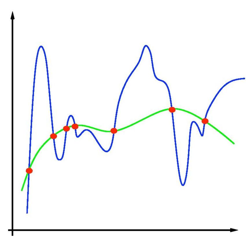
7 GRADIENT BOOSTING TO UNIFY ALL SIGNALS
Every component produces an important signal for the final matching decision, but in order to get
high accuracy, we also need to learn how important each of them is. For example, 95% match in
the name means that offer is very likely belonging to the product, but if many other signals say
that the offer should not match, it can mean that eshop provided incorrect title or that model
for title evaluation is faulty. Figure 22 shows part of one of the decision trees from the ensemble
trained using XGBoost, where f0 stands for the similarity between offer and product name and
f7-10 are various price outlier tests mentioned in section 5.2.
Figure 22: Match decision visualization using trees
As we can see from the figure, the main part of the matching decision is indeed product title,
as it is the most used node in the tree with various rules, and other nodes provide hints in cases
of uncertainty. It will be interesting to see how this tree changes with the addition of other deep
learning models.
8 RESULTS
8.1 DIFFERENT MODEL ARCHITECTURES
The best accuracy on the validation dataset was achieved by the Siamese CNN-LSTM. The com-
parison of individual architectures is shown in table 6 below. For computational time reasons,
30You can also read