Utah Education Funding Study - Summary 1: Phase 2 Visualized in Nine Key Findings
←
→
Page content transcription
If your browser does not render page correctly, please read the page content below
PHASE 2 REPORT

                                    Utah Education
                                    Funding Study
                                    Summary 1: Phase 2 Visualized
                                    in Nine Key Findings
                                    Over the past 30 years, K–12 enrollment in Utah has grown rapidly, from
                                    446,652 in 1990 to 704,600 in 2023, and is projected to continue increasing
                                    over the next five years.1 As the state’s student population expands in size, it is
                                    also becoming more racially and ethnically diverse. It is projected that within
                                    the school-age population (i.e., ages 5–17), the proportion of individuals identi-
                                    fying as non-White will grow from 25 percent as of 2015 to 42 percent in 2065. 2
                                    These demographic changes, combined with the effort to step back to study
                                    the state’s school funding system, suggest a need to identify how best to design
                                    a system that meets the evolving needs of students and ensure how best to use
The Utah Education Funding
Study, Phase 2 report is the        the state’s resources to achieve state goals.
culmination of this study and       With these changes in mind, it is imperative that the state’s funding system
examines costs and resource
                                    evolve in step with the dynamic needs of its student body and reflect the
allocation through a variety of
methods, with an emphasis on        alignment of resources to ensure their best use. As such, the Utah State Board
equal educational opportunity.      of Education (USBE) partnered with WestEd and Augenblick, Palaich, and
                                    Associates (APA) to study the current K–12 funding system and to determine
The study’s overall conclu-
sions and final policy recom-       the extent to which funding formulas meet their intended purposes, particu-
mendations are discussed in         larly with respect to ensuring “reasonably equal educational opportunities for
the associated summary docu-        all children” (Utah Code Annotated § 53F-2-103).
ment: Summary 2 — Overall
Conclusions.                        The following series of findings and associated charts explain key takeaways
                                    from the second phase of the study.
The recommendations are
also covered in more detail in
Summary 3—Recommendation 1,
Summary 4 —Recommendations          1 National Center for Education Statistics (NCES). (2020). Enrollment in public
2–4, and Summary 5 —                  elementary and secondary schools, by region, state, and jurisdiction: Selected
Recommendations 5 and 6.              years, fall 1990 through fall 2023. https://nces.ed.gov/programs/digest/d13/
                                      tables/dt13_203.20.asp
                                    2 Hollingshaus, M., Harris, E., & Perlich, P. S. (2019). Utah’s increasing diversity:
                                      population projections by race/ethnicity. University of Utah, David Eccles School
                                      of Business. https://gardner.utah.edu/wp-content/uploads/Utah-Projections-
                                      Race-Ethnicity-2019.pdf.

          ADA Compliant: 2/9/2021   Utah Education Funding Study | Phase 2                                                  1
THERE IS A LARGE RANGE IN LOCAL PROPERTY WEALTH ACROSS DISTRICTS IN UTAH, WITH THE
WEALTHIEST DISTRICT HOLDING MORE THAN 15 TIMES THE TAXABLE ASSESSED PROPERTY VALUE
PER AVERAGE DAILY MEMBERSHIP (FINDING 1).
Exhibit 7 from the report displays the taxable assessed property value (TAV) per average daily membership
(ADM), from lowest to highest, for all 41 school districts, along with the average value. There is a wide range in
property wealth among school districts. For example, the highest TAV per ADM, in Park City School District, is
more than 15 times greater than the lowest, in South Sanpete School District, and more than four times greater
than the average.
Exhibit 7. Taxable Assessed Property Value Per Average Daily Membership (in $1,000s)
by Utah School District in FY 2017–18
$3,500
Taxable Assessed Property Value Per ADM
$3,000
$2,500
$2,000
$1,500
$1,000
$500
$0
te
Uin ge
Mu on
Pro n
ga e
To e
Se e
Mo an
ity
Ga tah
Ca o
ne
y
r
Ca rray
Mi ch
le
W is
Em d
Da ich
ash Iron
Ca n e
Av ns
Pa e tt
Sa an
Alp e
Sa ery
te
de r
Jor ty
vo
W yne
Du ton
Bo eber
Gr ab
um it
Be e
t
So h Su nd
er
W ld
No San tic
vie
mi
b
Og Elde
rga
Cit
Lo anit
ut mm
ch
in
r
et
ak
Piu
v
oe
era
e
pe
i
lla
t
av
o
rb
nC
Ju
nC
d
Ka
Ne
Tin
es
rth Ju
Da
rt ra
R
gg
asa
np
rfi
ing
lt L
a
ny
rk
an
G
ch
x
hS
hS
W
ut
No
So
School Districts
Source: Authors’ calculations based upon FY 2017–18 data from the Utah State Tax Commission, Property Tax Division and
the USBE.
ALTHOUGH EQUALIZATION POLICIES ARE IN EFFECT, THE IMPACTS OF THESE POLICIES ON FISCAL
NEUTRALITY ARE LIMITED (FINDING 3).
Exhibit 10 from the report helps illustrate the equalization effect of state guarantee aid for voted levies, as of
FY 2017–18. Districts on the left end of the chart — those with the lowest TAV per ADM — receive, in some
cases, half or more of total voted levy revenue through state guarantee aid (51 percent on average). Districts
on the right end of the chart — those with the highest TAV per ADM — receive little or no state guarantee aid
(2 percent on average).
However, the data suggest that there are limits to the impact of the current state guarantee aid program. On
average, the tax rate among districts with TAV per ADM below the state median is higher than the tax rate among
districts with TAV per ADM above the median. However, the below-the-median districts generate less revenue
Utah Education Funding Study | Phase 2 2than their wealthier peers, with an average of $758 per ADM total revenue for districts below the median TAV per ADM, compared to $953 per ADM for districts above the median. Exhibit 10. Voted Local Levy and Local and State Aid Shares Per Average Daily Membership in FY 2017–18 Source: Authors’ calculations based upon FY 2017–18 data from the Utah State Tax Commission, Property Tax Division and the USBE. WHEN PUT IN COMPARABLE TERMS, STATE-REQUIRED TAX RATES THAT DEFINE THE LOCAL SHARE ARE MORE SIMILAR TO EACH OTHER THAN IT MIGHT SEEM, THOUGH UTAH’S IS THE SECOND LOWEST (FINDING 9). The study team also examined the amount of effort required by states that set a statutory mill levy, displayed in Exhibit 17 of the report, to consider how Utah’s Basic Property Tax Levy compares to other states. To be able to compare the amounts of required effort of each state’s tax rates, a few conversions were necessary. First, to ease interpretation, tax rates were converted to mills.3 Second, for each state for which data were available, state mill rates were converted into a mills per actual property value metric. This step is important because not all states create an assessed value based on 100 percent of the actual homestead property value for tax purposes. 4 In Utah, in general, taxable property value is based on 100 percent of the assessed value, but there is an exemp- tion for residential property, equal to a 45 percent reduction in the value, which is equivalent to 55 percent of the assessed value (Utah Code Annotated § 59-2-103). Although this exemption is not factored into the state 3 A common way to refer to tax rates, mills are the dollars of tax per $1,000 of assessed value, or the tax rate multiplied by 1,000. 4 For example, in Alabama, assessed value of homestead property is 20 percent of real property value, and the state requires 10 mills on homestead assessed value. Multiplying 10 mills times 20 percent of actual value generates a mills per actual value of 2 mills. Utah Education Funding Study | Phase 2 3
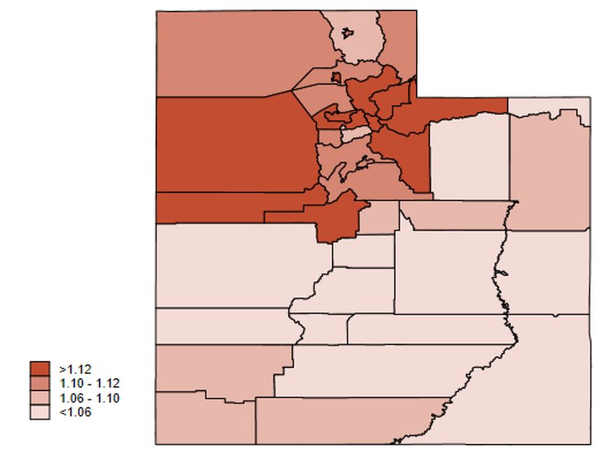
comparisons displayed in Exhibit 17, it should be noted that if this exemption were factored in, the mill per actual
value for Utah would decrease because less than 100 percent of the assessed value is taxable in some cases.

Exhibit 17. Mills Per Actual Property Value for States With Statutory Mills

 State                       Mill Rate                      Taxable Property Value         Mill per Actual Value

 Utah                        1.6                            100%                           1.6

 Alabama                     10                             20%                            2

 Arkansas                    25                             20%                            5

 Georgia                     5                              40%                            2

 Iowa                        5.4                            100%                           5.4

 Kansas                      20                             11.5%                          2.3

 Kentucky                    3                              100%                           3

 Mississippi                 28                             10%                            2.8

 Missouri                    34.3                           19%                            6.5

 Nebraska                    10.2                           100%                           10.2

 Nevada                      7.5                            35%                            2.6

 New Mexico                  .5                             33%                            0.2

 Oklahoma                    35                             12.5%                          4.4

 Texas                       9.3                            100%                           9.3

 Wyoming                     25                             9.5%                           2.4

Source: The study team examined the school finance systems of states to identify the mill rate and assessment percentages
for the state systems.

Fifteen states, including Utah, set a statutory mill rate to locally fund schools. The rates set in state statutes vary
greatly across states; however, once the rate is applied to the taxable property value, the mills per actual value
are generally comparable across states, with a few exceptions. Utah and New Mexico were the only states that
mandated less than 2 mills per actual value, at 1.6 and 0.2 mills, respectively.

LOCAL PRICES FOR TEACHER LABOR VARY GEOGRAPHICALLY, WITH PRICES UP TO 31 PERCENT
HIGHER IN SOME REGIONS, COMPARED TO OTHERS (FINDING 10).
This study analyzed differences in teacher salaries resulting to differences in a district’s location. The index
resulting from this analysis was the Teacher Salary Index (TSI). The TSI was created through a method known as
a hedonic wage analysis. This type of model seeks to predict teacher salaries when only factors that are out of a
district’s control are taken into account.

Utah Education Funding Study | Phase 2                                                                                 4
This index ranges from 1.00 to 1.31, indicating that with respect of differences of location the price of teacher
labor is estimated to be, at most, 31 percent higher in some parts of Utah than in others.
To illustrate geographic variation in the price of labor, Exhibit 19 from the report displays the average district-level
TSI in the most recent year of analysis, FY 2018–19. As shown in Exhibit 19, the price of teacher labor is highest in the
districts in the northwestern part of the state, generally clustered around the Salt Lake City metro area.

Exhibit 19. Map of the Average District-Level Teacher Salary Index, FY 2018–19

Source: Authors’ calculations based on the data used for the hedonic wage analysis, described in detail in the full report.

HIGHER SPENDING IS PREDICTED AS SCHOOL AVERAGE ACADEMIC GROWTH INCREASES, THOUGH
THIS ASSOCIATION IS LOWER IN MAGNITUDE AMONG HIGH SCHOOLS, COMPARED TO NON–HIGH
SCHOOLS (FINDING 11).
An important and common question in education finance literature is whether increases in spending can truly
affect student outcomes. The cost function analysis is one approach to understanding the extent of the associa-
tion between spending and outcomes. However, it cannot speak to whether one is causing the other. 5
Nonetheless, a cost function analysis provides important information about whether, in a particular state context,
policymakers can view investments in education as supporting improvements to student outcomes on average,
given the factors accounted for in the analysis.
As shown in Exhibit 20, in the Utah cost function analysis, higher spending is predicted as school average academic
growth increases. When considering only high schools, the rate of growth is smaller, but is still significantly positive.

5 For example, if a particular set of high-performing schools is found to be spending more after accounting for cost
  factors, this finding should not be interpreted as evidence that the spending is causing the outcomes.

Utah Education Funding Study | Phase 2                                                                                        5
This finding is remarkably consistent with other recent cost function analyses.6 For example, in a recent cost func-
tion analysis in North Carolina,7 the magnitude of the relationship is comparable to the one found in Utah, and a
similar trend is observed with respect to this relationship in high schools, compared to non–high schools.
Although comparisons of cost function analyses conducted in different states should be made with some caution,
this level of consistency in results provides important support for the finding in general.

It may be helpful to briefly explain this and the other graphics presented here. For findings
11 through 13 and 15, a scatterplot is presented that illustrates, on the y-axis, the predicted
spending relative to the minimum predicted spending when only the variable of interest is
allowed to vary and all other variables are held constant. The x-axis displays the value of
the variable of interest for each school, in ascending order. In Exhibit 20, the x-axis is the
measure of academic growth, school-level average normal curve equivalent scores, and
the y-axis is the predicted spending above the minimum. As academic growth increases,
predicted spending increases, as indicated by the upward-sloping trend.

Exhibit 20. Student Outcomes Results — Academic Growth

                                          5
Predicted Cost Compared to the Baseline

                                          4

                                          3

                                          2

                                          1
                                              0.2   0.4                      0.6                         0.8                                1
                                                                 School-level Avg. NCE Score

                                                          High School    Not High School

Source: Authors’ calculations based on the data used for the cost function analysis, described in detail in the full report.

6 E.g., Taylor, L., Willis, J., Berg-Jacobson, A., Jaquet, K., & Caparas, R. (2018). Estimating the costs associated with reaching
  student achievement expectations for Kansas public education students. WestEd; Willis, J., Krausen, K., Berg-Jacobson, A., Taylor, L.,
  Caparas, R., Lewis, R., & Jaquet, K. (2019). A study of cost adequacy, distribution, and alignment of funding for North Carolina’s K–12
  public education system. WestEd.
7 Willis, J., Krausen, K., Berg-Jacobson, A., Taylor, L., Caparas, R., Lewis, R., & Jaquet, K. (2019). A study of cost adequacy,
  distribution, and alignment of funding for North Carolina’s K–12 public education system. WestEd.

  Utah Education Funding Study | Phase 2                                                                                                    6
HIGHER SPENDING IS ALSO PREDICTED AS SCHOOL GRADUATION RATE INCREASES (FINDING 12). In the context of cost function analysis, results of previous, recent cost function analyses with respect to gradu- ation rate as a measure of student outcomes are generally more mixed. In some studies, positive and significant associations are found, 8 while in another the results are insignificant, suggesting that, in that case, additional spending had no clear association with improvements in graduation rates. 9 A variety of factors may explain these differences in the results of these previous studies. Most generally, observ- able and unobservable factors may impact the extent to which spending is differently associated with graduation in different states. Despite the apparent general challenges with graduation rate as an outcome measure in the context of prior cost function analysis modeling, this study’s analysis found that spending is predicted to increase as graduation rates increase, as displayed in Exhibit 21 of the report, and that this result is statistically significant. Exhibit 21. Student Outcomes Results — Graduation Rate Source: Authors’ calculations based on the data used for the cost function analysis, described in detail in the full report 8 See Taylor, L., Willis, J., Berg-Jacobson, A., Jaquet, K., & Caparas, R. (2018). Estimating the costs associated with reaching student achievement expectations for Kansas public education students. WestEd; Willis, J., Doutre, S. M., & Berg-Jacobson, A. (2019). Study of the individualized education program (IEP) process and the adequate funding level for students with disabilities in Maryland. WestEd. 9 Willis, J., Krausen, K., Berg-Jacobson, A., Taylor, L., Caparas, R., Lewis, R., & Jaquet, K. (2019). A study of cost adequacy, distribution, and alignment of funding for North Carolina’s K–12 public education system. WestEd. Utah Education Funding Study | Phase 2 7
PREDICTED SPENDING GENERALLY DECREASES AS DISTRICT ENROLLMENT INCREASES, PROVIDING
EVIDENCE THAT ECONOMIES OF SCALE ARE PRESENT IN UTAH AT THE DISTRICT LEVEL (FINDING 13).
A commonly observed phenomenon in economic literature is that as organizations grow in scale, per-unit costs
decline, except, in some cases, in organizations of a very large scale. This phenomenon is generally referred to
as economies of scale. Conceptually, this makes sense. Very small organizations likely must establish the same
foundational elements in order to begin operating. Beyond foundational costs, there is also some cost per every
additional unit of production, the total of which changes as the scale of production changes. In small organizations,
the fixed foundational costs make up a larger share of costs and reflect a larger per-unit cost, compared to larger
organizations, for which these foundational costs are a small proportion of the total.
In the education context, this is perhaps best illustrated in staffing costs. A district serving 150 students must
still hire a sufficient number of teachers to staff all grades that it serves, even if some only serve a handful of
students. In this case, the per-pupil spending for each school will be twice that of a district that serves twice as
many students and that can hire the same configuration of staff.
As illustrated by Exhibit 22 of the report, predicted spending decreases as district enrollment increases, suggesting
economies of scale.

Exhibit 22. District Scale of Operations Results
                                       3.5
 Predicted Cost Compared to Baseline

                                        3

                                       2.5

                                        2

                                       1.5

                                        1
                                             50   500                          5,000                        50,000
                                                         District Enrollment

Source: Authors’ calculations based on the data used for the cost function analysis, described in detail in the full report.

PREDICTED SPENDING INCREASES AS THE LEVEL OF STUDENT NEED INCREASES, AS MEASURED
BY THE PERCENTAGES OF ECONOMICALLY DISADVANTAGED STUDENTS AND STUDENTS WITH
DISABILITIES (FINDING 15).
Another critical factor in the cost of education is the level of need among a school’s population of students. It is widely
understood that students’ innate characteristics and access to out-of-school resources influence the resources
required within the public-school setting to ensure that all students have equivalent educational opportunities.

Utah Education Funding Study | Phase 2                                                                                         8
The school-level proportions of economically disadvantaged (ED) students and of students identified for an individu-
alized education plan (IEP) are included in this study’s analysis. Although these measures do not encompass every way
in which a student’s needs impact a school’s costs, they are thought to encompass the aspects of a student that most
strongly influence cost, that are correlated with other measures of need, and that improve the model estimates.10
In alignment with prior studies,11 the study team found that, as shown in Exhibit 24 of the report, as the level of
student need rises, spending is predicted to also rise when student outcomes and cost factors are held constant.
Exhibit 24. Student Needs – Economically Disadvantaged Students and Students With IEPs
Predicted Cost Compared to Baseline
1.4
1.3
1.2
1.1
1
0 0.1 0.2 0.3 0.4 0.5 0.6 0.7 0.8 0.9 1
School-level EDS (%)
2
Predicted Cost Compared to Baseline
1.8
1.6
1.4
1.2
1
0 0.1 0.2 0.3 0.4
School-level SPED (%)
Source: Authors’ calculations based on the data used for the cost function analysis, described in detail in the full report.
10 The exclusion of English learners from the set of student need measures requires some explanation. It is because,
in Utah, the status of students as ED is very strongly correlated with their status as an English learner. A relationship
this strong can pose a problem because if two factors are strongly correlated enough, their unique effects can be
hard to estimate separately without bias. Given this issue, it is best to view the results with respect to ED students as
also reflecting a general finding for English learners. The English learner population and the ED student population
overlap to such a great extent that resources dedicated to one are likely to benefit the other, especially in the few Utah
communities with large populations of English learners.
11 E.g., Duncombe, W. D., & Yinger, J. (2005). How much more does a disadvantaged student cost? Center for Policy Research at
Syracuse University; Taylor, L., Willis, J., Berg-Jacobson, A., Jaquet, K., & Caparas, R. (2018). Estimating the costs associated with reaching
student achievement expectations for Kansas public education students. WestEd; Willis, J., Krausen, K., Berg-Jacobson, A., Taylor, L.,
Caparas, R., Lewis, R., & Jaquet, K. (2019). A study of cost adequacy, distribution, and alignment of funding for North Carolina’s K–12
public education system. WestEd.
Utah Education Funding Study | Phase 2 9PROGRAMS EXPLICITLY TARGETING “AT-RISK” STUDENTS OR ECONOMICALLY DISADVANTAGED STUDENTS PROVIDE SIGNIFICANTLY LESS ADDITIONAL FUNDING THAN WOULD BE PROVIDED UNDER THE WEIGHT DERIVED FROM THE COST FUNCTION ANALYSIS (FINDING 20). To assess the current level of investment in additional resources for “at-risk” and ED students, the study team first considered the overall level of resources in operational expenditures dedicated to five selected programs that target funds to these populations, as displayed in Exhibit 31 of the report. At about $95.8 million total, these existing programs add up to a minimal amount of spending when compared to all operational expenditures (~$4.4 billion). Assuming that all of the dollars for these programs are targeted to “at-risk” students, this amount of spending represents an additional $187 per “at-risk” pupil. Exhibit 31. Student Funding: Selected Programs and Overall Operational Expenditures, FY 2018–19 Program Total (in millions) Per-Pupil Per “At-Risk” Pupil Overall Operational 4,400 7,073 N/A Expenditures Enhancement for At-Risk 41.9 67 82 Students Early Intervention 8.5 14 17 Program Early Literacy Program 43.5 70 85 Partnership for Student 1.2 2 2 Success Intergenerational Poverty 0.70 1 1 Interventions Total Among Selected 95.8 154 187 Programs Source: Authors’ calculations based on the data used for the cost function analysis, described in detail in the full report. Note: Values reported are approximate. Utah Education Funding Study | Phase 2 10
Exhibit 32 of the report displays the weight derived from the cost function analysis alongside two effective
weights: the weight based on Enhancement for At-Risk Students (EARS) funding alone, and the weight based on
all selected programs in Exhibit 31.

Exhibit 32. Comparing Weights Based on At-Risk Population

 Cost Function                            EARS Only                                 All Selected Programs
 Analysis Weight                          (“at-risk”)                               (“at-risk”)

 0.42                                     0.01                                      0.03

Source: Authors’ calculations based on the data used for the cost function analysis, described in detail in the full report.
Note: Values reported are approximate.

As indicated in Exhibit 32, the current level of resources implies an effective weight of only 0.03, which is well below
the weight derived from the cost function analysis. This effective weight being far below either of the comparison
weights reflects the fact that Utah currently explicitly targets very little spending to “at-risk” students.

Utah Education Funding Study | Phase 2                                                                                  11
You can also read