Very Large Telescope Paranal Science Operations VIRCAM/VISTA User Manual
←
→
Page content transcription
If your browser does not render page correctly, please read the page content below
EUROPEAN SOUTHERN OBSERVATORY
           Organization Européene pour des Recherches Astronomiques dans l’Hémisphère Austral
           Europäische Organization für astronomische Forschung in der südlichen Hemisphäre

           ESO - European Southern Observatory
           Karl-Schwarzschild Str. 2, D-85748 Garching bei München

                Very Large Telescope
             Paranal Science Operations
             VIRCAM/VISTA User Manual

                           Doc. No. VIS-MAN-ESO-06000-0002

                                  Issue 108, Date 01/06/2021

      V. D. Ivanov, T. Szeifert, B. Häußler
Prepared . . . . . . . . . . . . . . . . . . . . . . . . . . . . . . . . . . . . . . . . . . . . . . . .
                                                                Date                    Signature

                              C. Dumas
Approved . . . . . . . . . . . . . . . . . . . . . . . . . . . . . . . . . . . . . . . . . . . . . . . .
                                                                Date                    Signature

                             A. Kaufer
Released . . . . . . . . . . . . . . . . . . . . . . . . . . . . . . . . . . . . . . . . . . . . . . . .
                                                                 Date                   Signature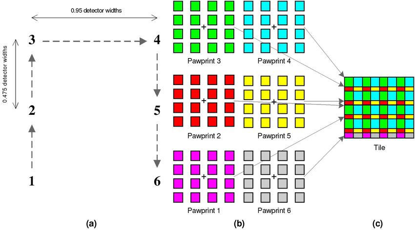
ii   VIRCAM/VISTA User Manual                    VIS-MAN-ESO-06000-0002

        This page was intentionally left blank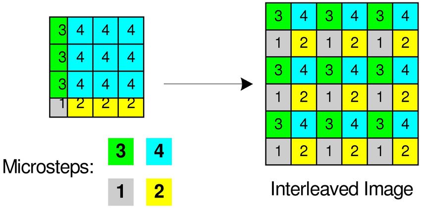
VIRCAM/VISTA User Manual                   VIS-MAN-ESO-06000-0002                                iii

                                         Change Record

 Issue     Date       Section affected                    Reason/Initiation/Documents/Remarks

 0.10    09/09/2008   All                                 Creation, V. D. Ivanov & VISTA Project Office
 1.00    18/12/2009   All                                 First public release for P85.
 1.01    01/07/2010   All                                 Update for P86 Phase II and P87 Phase I.
 1.02    01/12/2010   Twilight, overheads.                Update P87 Phase II.
 1.03    11/03/2011   Minor updates.                      Update P88 Phase I.
 1.04    04/08/2011   Web links updated.                  Update P89 Phase I.
 1.05    13/06/2013   Template tile6sky info.             Update P92 Phase II.
 1.06    29/08/2013   Minor updates.                      Update P93 Phase I.
 1.07    25/11/2013   ToO description.                    Update P93 Phase II.
 1.08    13/03/2018   Minor updates (p2pp to p2)          Update P101.
 1.09    12/05/2018   Minor updates Table 1, typos, etc   Update P106
 1.10    01/06/2021   update on USD contact               Update P108
iv   VIRCAM/VISTA User Manual                    VIS-MAN-ESO-06000-0002

        This page was intentionally left blank
VIRCAM/VISTA User Manual                       VIS-MAN-ESO-06000-0002                                                                                  v

Contents

1 Introduction                                                                                                                                        1

2 Applicable documents and other sources of information                                                                                                3

3 Abbreviations and Acronyms                                                                                                                           5

4 VISTA and VIRCAM in a nut-shell                                                                                                                      6

5 The VISTA Telescope – Technical Description                                                                                                          7

6 The VIRCAM - VISTA Infra-Red Camera                                                                                                                  9
  6.1 General features . . . . . . . . . . . . . . . . .      .   .   .   .   .   .   .   .   .   .   .   .   .   .   .   .   .   .   .   .   .   .    9
  6.2 Detectors . . . . . . . . . . . . . . . . . . . . .     .   .   .   .   .   .   .   .   .   .   .   .   .   .   .   .   .   .   .   .   .   .   11
  6.3 Filters . . . . . . . . . . . . . . . . . . . . . . .   .   .   .   .   .   .   .   .   .   .   .   .   .   .   .   .   .   .   .   .   .   .   16
  6.4 Sensitivity . . . . . . . . . . . . . . . . . . . . .   .   .   .   .   .   .   .   .   .   .   .   .   .   .   .   .   .   .   .   .   .   .   19
  6.5 Low Order Wavefront Sensors and Autoguiders             .   .   .   .   .   .   .   .   .   .   .   .   .   .   .   .   .   .   .   .   .   .   20
  6.6 High Order Wavefront Sensor Operation . . . .           .   .   .   .   .   .   .   .   .   .   .   .   .   .   .   .   .   .   .   .   .   .   21

7 Observations with VIRCAM@VISTA                                                                                                                      25
  7.1 Observations in the Infrared . . . . . . . . . . . . . . . . . . . . . . . . . . . . . . . .                                                .   25
      7.1.1 The Infrared Sky . . . . . . . . . . . . . . . . . . . . . . . . . . . . . . . . . .                                                  .   25
      7.1.2 Selecting the best DIT and NDIT . . . . . . . . . . . . . . . . . . . . . . . . .                                                     .   26
  7.2 Preparation for observations and general operation of VIRCAM@VISTA . . . . . . .                                                            .   27
      7.2.1 Target of Opportunity (ToO) observations . . . . . . . . . . . . . . . . . . . .                                                      .   28
  7.3 Twilight Constraints . . . . . . . . . . . . . . . . . . . . . . . . . . . . . . . . . . . . .                                              .   29
  7.4 Pawprints, Tiles, Jitters, Microsteps . . . . . . . . . . . . . . . . . . . . . . . . . . . .                                               .   32
      7.4.1 Definitions . . . . . . . . . . . . . . . . . . . . . . . . . . . . . . . . . . . . . .                                               .   32
      7.4.2 “Filling-in” a tile with multiple pawprints . . . . . . . . . . . . . . . . . . . . . .                                               .   33
  7.5 Scheduling Containers . . . . . . . . . . . . . . . . . . . . . . . . . . . . . . . . . . .                                                 .   35
  7.6 Observing Strategy, Nesting . . . . . . . . . . . . . . . . . . . . . . . . . . . . . . . .                                                 .   36
  7.7 Autoguiding and AO operation . . . . . . . . . . . . . . . . . . . . . . . . . . . . . .                                                    .   38
  7.8 Overheads . . . . . . . . . . . . . . . . . . . . . . . . . . . . . . . . . . . . . . . . .                                                 .   38
  7.9 Calibration Plan . . . . . . . . . . . . . . . . . . . . . . . . . . . . . . . . . . . . . . .                                              .   39
      7.9.1 Instrument signature removal . . . . . . . . . . . . . . . . . . . . . . . . . . .                                                    .   40
      7.9.2 Photometric Calibration . . . . . . . . . . . . . . . . . . . . . . . . . . . . . .                                                   .   43
      7.9.3 Astrometric Calibration . . . . . . . . . . . . . . . . . . . . . . . . . . . . . .                                                   .   45
      7.9.4 Additional Calibrations Derived from Science Data and Related Observing
              Strategies . . . . . . . . . . . . . . . . . . . . . . . . . . . . . . . . . . . . . .                                              . 46

8 Data Flow, Pipeline, Quality Control                                                                                                                50

9 References and Acknowledgments                                                                                                                      54

A VISTA/VIRCAM Template Reference                                                               55
  A.1 Historic P86 Modifications of the Templates (Oct. 2010) . . . . . . . . . . . . . . . . . 55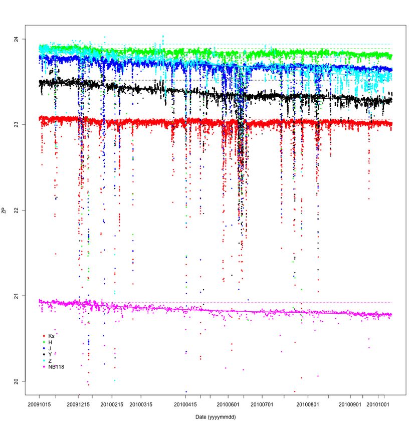
vi                           VIRCAM/VISTA User Manual                      VIS-MAN-ESO-06000-0002

     A.2 Historic P85 Modifications of the Templates (Feb. 2010) . . . . . . . . . . . . . . . .     .   55
     A.3 Introduction to the Phase 2 Preparation for Public Surveys . . . . . . . . . . . . . . .    .   55
     A.4 The Acquisition Templates – VIRCAM img acq tile and VIRCAM img acq quick . . .              .   57
     A.5 The Science Observation Templates . . . . . . . . . . . . . . . . . . . . . . . . . . .     .   59
         A.5.1 VIRCAM img obs tile . . . . . . . . . . . . . . . . . . . . . . . . . . . .        .   59
         A.5.2 VIRCAM img obs tile6sky . . . . . . . . . . . . . . . . . . . . . . . . . . . . .     .   66
         A.5.3 VIRCAM img obs paw . . . . . . . . . . . . . . . . . . . . . . . . . . . . . .        .   66
     A.6 The Calibration Templates – VIRCAM img cal illumination and VIRCAM img cal std              .   68
     A.7 Template Parameter Tables . . . . . . . . . . . . . . . . . . . . . . . . . . . . . . . .   .   68

B VISTA/VIRCAM Observing Blocks Cookbook                                                                 74

C VISTA@VIRCAM FITS Header Description                                                                   76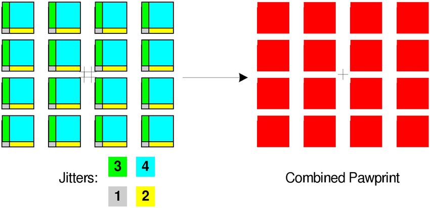
VIRCAM/VISTA User Manual                             VIS-MAN-ESO-06000-0002                                         1

1        Introduction

VISTA or Visible1 and Infrared Survey Telescope for Astronomy is a specialized 4-m class wide field
survey telescope for the Southern hemisphere. VISTA is located at ESO Cerro Paranal Observatory
in Chile (longitude 70o 23’ 51”W, latitude 24o 36’ 57” S, elevation 2500 m above sea level) on its own
peak about 1500 m N-NE from the Very Large Telescope (VLT).
The telescope has an alt-azimuth mount, and quasi-Ritchey-Chretien optics with a fast f/1 primary
mirror giving an f/3.25 focus ratio at the Cassegrain focus. It is equipped with a near infrared camera
VIRCAM or VISTA InfraRed Camera (with a 1.65 degree diameter field of view (FOV) at VISTA’s
nominal pixel size) containing 67 million pixels of mean size 0.339 arcsec × 0.339 arcsec. The
instrument is connected to a Cassegrain rotator on the back of the primary mirror cell, and has
a wide-field corrector lens system with three infrasil lenses. The available filters are: broad band
ZY JHKS and narrow band filter at NB 980, NB 990, and 1.18 micron. The point spread function
(PSF) of the telescope+camera system delivers images with a full width at half maximum (FWHM)
of ∼0.51 arcsec (without the seeing effects). The weather characteristics and their statistics are
similar to those for the VLT.
VISTA has one observing mode - imaging - and the telescope is used mostly in service mode to carry
out surveys - programs exceeding in size and scope the usual ESO Large Programs. Typically, the
observations are carried out in a 6-step pattern, called tile, designed to cover the gaps between the
individual detectors.
The high data rate (on average 315 GB per night) and the large size of the individual files (256.7 MB)
makes it a significant challenge for an individual user to cope with the data reduction challenges.
The VISTA raw data are available via the ESO archive. High-level data products (i.e. photometry,
catalog with object classification and derived physical parameters, etc.) are also available via the
ESO archive for the ESO Public Surveys.
This manual is divided into several sections, including a technical description of the telescope and
the camera, a section devoted to the observations with VISTA, including general information about
the nature of the infrared sky, the operation of VISTA, the sensitivity of the instrument and a cali-
bration plan. Next, the manual summarizes the data flow, the pipeline, and the parameters that are
used for the quality control. Finally, the Appendix contains a template reference guide.
This manual was based on many documents, kindly provided by the VISTA consortium. The authors
hope that you find it useful in your VISTA observations. The manual is continuously evolving with
the maturing of the telescope and there will always be room for improvement. Comments from the
users are especially welcomed. Please, refer to the ESO VISTA web site for contact details.

Nota Bene:

        • The web page dedicated to VIRCAM/VISTA is accessible from the La Silla Paranal Observa-
          tory home page at: http://www.eso.org/sci/facilities/paranal/instruments/vircam/
          You will find there the most up-to-date information about VIRCAM/VISTA, including recent
          news, efficiency measurements and other useful data that do not easily fit into this manual or
    1
   A wide field visible camera was considered during the early stages of VISTA development, accounting for the visible
component to the telescope name.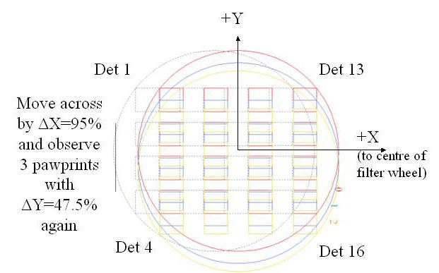
2                          VIRCAM/VISTA User Manual                      VIS-MAN-ESO-06000-0002

      is subject of frequent changes. This web page is updated regularly.
      An external (with respect to ESO) source with history of the project and relevant information is
      the VISTA consortium web-page at: http://www.vista.ac.uk/index.html

    • Please, read the latest User Manual! It is located at:
      http://www.eso.org/sci/facilities/paranal/instruments/vircam/doc/

    • Contact information: for questions about VISTA and VIRCAM write to vista$@$eso.org.
      Should you have questions, please check out our Operations Helpdesk at https://support.
      eso.org where you can browse our knowledgebase and contact us through the dedicated
      form. This tool is available at the start of Phase 2 for P108.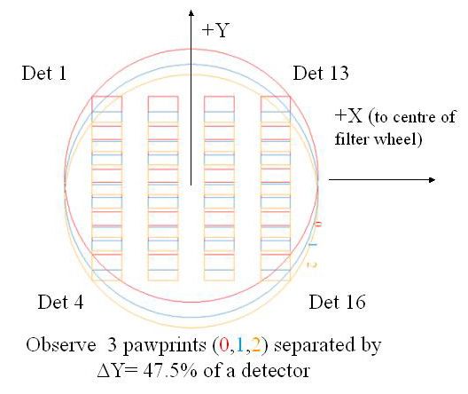
VIRCAM/VISTA User Manual                VIS-MAN-ESO-06000-0002                        3

2    Applicable documents and other sources of information

Documents:

    • VLT-MAN-ESO-00000-0000 OS Users’ Manual

    • VLT-MAN-ESO-00000-0000 DCS Users’ Manual

    • VLT-MAN-ESO-00000-0000 ICS Users’ Manual

    • VLT-MAN-ESO-00000-0000 SADT Cookbook

Web sites:

    • ESO VIRCAM/VISTA main page:
      http://www.eso.org/sci/facilities/paranal/instruments/vircam/

    • VIRCAM/VISTA operation team contact list:
      http://www.eso.org/sci/facilities/paranal/instruments/vircam/iot.html

    • ESO Public Surveys:
      http://www.eso.org/sci/observing/PublicSurveys.html

    • ESO VIRCAM/VISTA Quality Control:
      http://www.eso.org/observing/dfo/quality/index_vircam.html

    • ESO Data Archive: http://archive.eso.org/cms/

    • ESO P2: https://www.eso.org/p2/
      https://www.eso.org/sci/observing/phase2/p2intro.VIRCAM.html

    • ESO SADT page: http://www.eso.org/sci/observing/phase2/SMGuidelines/SADT.html
      http://www.eso.org/sci/observing/phase2/SMGuidelines/SADT.VIRCAM.html

    • VIRCAM/VISTA Science Archive (at ROE): http://horus.roe.ac.uk/vsa

    • VIRCAM/VISTA Science Verification: http://www.eso.org/sci/activities/vistasv.html

    • VIRCAM/VISTA Consortium: http://www.vista.ac.uk/index.html

    • VIRCAM/VISTA at UK Astronomy Technology Centre:
      https://www.roe.ac.uk/atc/projects/vista/

    • Cambridge Astronomical Survey Unit (CASU): http://casu.ast.cam.ac.uk/
      http://www.ast.cam.ac.uk/$\sim$mike/casu/index.html

    • VIRCAM/VISTA Data Flow System (VDFS; at CASU): http://www.ast.cam.ac.uk/vdfs/
      www.maths.qmul.ac.uk/$\sim$jpe/vdfs/

    • Wide Field Astronomy Unit (WFAU): http://www.roe.ac.uk/ifa/wfau/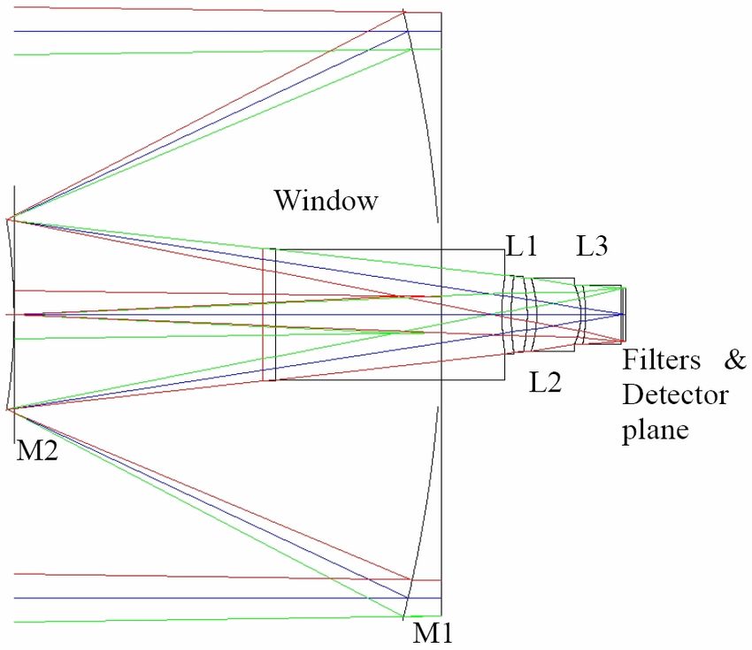
4                        VIRCAM/VISTA User Manual                 VIS-MAN-ESO-06000-0002

    • Astronomical Wide-field Imaging System for Europe (Astro-WISE): http://www.astro-wise.
      org/

    • Deep Near Infrared Survey of the Southern Sky (DENIS):
      http://cdsweb.u-strasbg.fr/denis.html

    • The Two Micron All Sky Survey (2MASS; at IPAC): http://www.ipac.caltech.edu/2mass/

    • UKIRT IR Deep Sky Survey: http://www.ukidss.org/
VIRCAM/VISTA User Manual VIS-MAN-ESO-06000-0002 5
3 Abbreviations and Acronyms
The abbreviations and acronyms used in this manual are described in Table 1.
Table 1: Abbreviations and Acronyms used in this manual.
ADU Analog-Digital Units MINDIT Minimum DIT ( = 1.0011 sec)
AG Autoguider NDIT Number of DITs
AO Adaptive Optics NDR Non-Destructive Read
BOB Broker of Observing Blocks NINT Number of NDITs
CDS Correlated Double Sample NTT New Technology Telescope
(IR detector readout mode) OB Observing Blocks
CP Cryo-pump OS Observing Software
DFS Data Flow System OT Observing Tool
DAS Detector Acquisition System P2 Phase 2 web tool for Proposal Preparation
DCR Double Correlated Read PSC Point Source Catalog
DCS Detector Control System PDU Power Drive Unit
DEC Declination PSF Point Spread Function
DIT Detector Integration Time RA Right Ascension
ESO European Southern Observatory QC Quality Control
ETC Exposure Time Calculator RON Read Out Noise
FCA Force Control Assembly SADT Survey Area Definition Tool
FITS Flexible-Image Transport System SM Service Mode
FOV Field Of View SOFI Son Of ISAAC
FPA Focal Plane Assembly TBC To Be Confirmed
FWHM Full Width at Half Maximum TCS Telescope Control System
GFRP Glass Fibre Reinforced Plastic TSF Template Signature File
HOWFS High Order Wave Front (curvature) Sensor UKIRT United Kingdom Infrared Telescope
ICRF International Coordinate Reference Frame VDFS VISTA Data Flow System
ICRS International Celestial Reference System VIRCAM VISTA InfraRed Camera
ICS Instrument Control System VISTA Visual and IR Survey Telescope for Astronomy
IR Infra-Red VLT Very Large Telescope
ISAAC IR Spectrograph And Array Camera VM Visitor Mode
LOCS Low Order Curvature Sensors VST VLT Survey Telescope
LOWFS Low Order Wave Front (curvature) Sensor VPO VISTA Project Office
(same as LOCS) WCS World-Coordinate System
LCU Local Control Unit WFCAM Wide-Field Camera (IR camera at UKIRT)
M1 Primary Mirror ZP Zero Point
M2 Secondary Mirror ZPN Zenithal Polynomial (Projection)
MAD Median of Absolute Deviation6 VIRCAM/VISTA User Manual VIS-MAN-ESO-06000-0002
4 VISTA and VIRCAM in a nut-shell
A summary of basic VISTA and VIRCAM related terms and concepts is given in Table 2.
Table 2: Short telescope and instrument description.
Item Description
Telescope VISTA a specialized 4-m telescope for surveys
Instrument VIRCAM wide field 16 detector near-infrared camera
Location VISTA peak at ESO Paranal Observatory
(Latitude S24 37.5, Longitude W70 24.2, Altitude above
sea level 2635.43 m)
Focus f/1 primary giving a f/3.25 focus at the Cassegrain
Observing mode imaging
Detectors 16 Raytheon VIRGO 2048 px×2048 px (HgCdTe on
CdZnTe substrate) arrays
Total number of pixels 64 megapixels
Pixel size square, average 0.339 arcsec on the side; for more
details on the variation see Sec. 7.9.3
Image quality FWHM=0.51 arcsec
Filters ZY JHKS , NB 980, NB 990, and NB 118
Integration a simple snapshot, within the Data Acquisition System,
of a specified Detector Integration Time
Exposure the stored product in a file, a sum (not an average!) of
many individual detector integrations
Pawprint the 16 non-contiguous images of the sky produced by
VIRCAM, with its 16 non-contiguous chips.
Tile a contiguous area of sky obtained by combining multiple
offsetted pawprints (filling in the gaps in a pawprint)
FOV of a single pawprint ∼0.6 deg2 , with gaps
FOV of a tile ∼1.64 deg2 filled FOV, obtained with a minimum of 6
exposures
Intradetector gaps 90% and 42.5% of the detector width
Image file size 256.7 MB
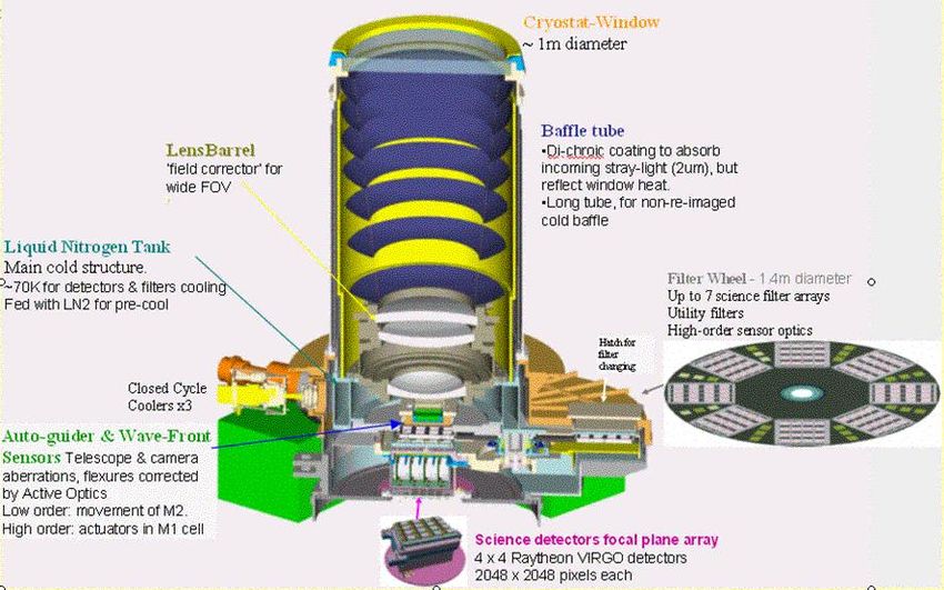
Nightly data rate 250 GB, peaking up to 600 GBVIRCAM/VISTA User Manual VIS-MAN-ESO-06000-0002 7 5 The VISTA Telescope – Technical Description VISTA is a 4-m class wide field survey telescope (Figure 1). It has an alt-azimuth mount, and quasi-Ritchie-Chretien optics with a 4.10-m fast f/1 primary mirror (M1) giving an f/3.25 focus at the Cassegrain. The f/3 hyperboloid-shaped secondary (M2) has a diameter of 1.24-m. The unvi- gnetted field of view is 2 deg (but VIRCAM uses only ∼1.6 deg). The entrance pupil has a diameter of 3.70-m. The focal length is 12.072-m. The mirrors were coated with silver at the start of the VIR- CAM operations in 2008, because was optimal for near-infrared performance. However, the silver coating suffered from fast aging so it was replaced with aluminum coating in 2011, and the current version of the VIRCAM ESO ETC reflects this change. The total telescope mass (above the foundation peer) is ∼113 metric tons, distributed among the optical support structure (∼44), the azimuth rotation structure (∼46) and the pedestal assembly (∼23). The primary mirror weights 5520 kg, the VIRCAM – 2900 kg, the secondary mirror – 1000 kg. The telescope has three Power Drive Units (PDU) enabling movement of the azimuth and altitude axis, and the Cassegrain rotator. Unlike most other telescopes, VISTA lies on a ball bearing with a pitch diameter of 3658 mm, instead on a oil bed. The Altitude limit is ≥20 deg above the horizon, which implies a mechanical pointing limit to the North at δ≤+45 deg at the meridian. The VISTA theoretical pointing error over the entire sky is 0.5 arcsec. The open-loop tracking error over 5 min of observation is 0.22-0.24 arcsec. The telescope can operate under humidity of up to 80%. when the temperature is within the operational temperature range of T=0–15 C. VISTA can not observe within 2 deg from the zenith because of a rotator speed limitation. The “jitter” movements are accomplished by moving the entire telescope (unlike the UKIRT for ex- ample, where this can be done via the tip-tilt mechanism of the secondary mirror). The overheads due to moving the telescope are 8 sec for a jitter, 15 sec for a pawprint, on average. The optical layout of the telescope is shown in Figure 2. The telescope and the instrument should be treated as one integral design, i.e. the telescope is just foreoptics to the VIRCAM. The design is intertwined to the point that the telescope guider is part of the camera, i.e. it is within the camera dewar. The primary mirror is manufactured from zerodur. Axial support is provided by 81 Force Control Assemblies (FCAs), mounted on the M1 cell, lateral support is carried out by four FCAs. The M2 position is controlled in 5 axis by a precision hexapod. VIRCAM is connected to the telescope via a rotator on the back of the primary mirror cell, and has a wide-field corrector lens system with three infrasil lenses. The camera is described in the next section. The enclosure rotates at nominal speed of 2 deg per second and is able to stop rotation within 5 sec. It can survive wind speed of up to 36 m s−1 closed. The nominal wind speed observing restrictions are: closing the dome at ≥18 m s−1 and observing at least 90 deg away from the wind direction for ≥12 m s−1 . The mirror coating is a major operation requiring dismounting of VIRCAM and the mirrors, and it implies interrupting the telescope operations for ∼10 days.
8                         VIRCAM/VISTA User Manual                     VIS-MAN-ESO-06000-0002

                         Figure 1: VISTA general view (CG - Cassegrain).

Figure 2: Optical layout of the telescope. M1 and M2 are the telescope primary and secondary
mirrors. The camera’s entrance window, the three lenses L1, L2, and L3, the filter and the detector
planes are also marked.
VIRCAM/VISTA User Manual VIS-MAN-ESO-06000-0002 9 6 The VIRCAM - VISTA Infra-Red Camera 6.1 General features The infrared camera VIRCAM (Figure 3) is a state-of-the art design, the largest of its kind, as of 2010. It has a very wide field of view with 1.65 deg diameter. The camera uses a long cryostat with seven nested cold baffles to block out-of-beam radiation instead of the usual re-imaging optics or cold pupil stop design that has been most common so far. In addition, the baffles serve to reject the unwanted heat load from the window by means of a specialized coating which is highly absorbing at wavelengths shortward of 3 µm and highly reflective longward of 3 µm. The baffling system still leaves a smooth gradient caused by scattered thermal radiation across the detectors in the KS band; the total intensity of this scattered background is expected to be ∼20% of the sky level and the gradient may be up to 10% of that, i.e. ∼2% of total sky level, including the “real” sky emission and the scattered light. This effect must be addressed during the data processing. On the positive side, the absence of a cold stop means that there is no intermediate focus, so there should be no issue with “nearly in focus” warm dust particles. The aluminum cryostat housing the camera consists of four main sections, and includes over 10-m of O-ring seals. The nominal vacuum level is 10−6 milibar, and it is achieved in two stages: an initial pump-down with an external pump followed by pumping with a pair of He closed cycle cryopumps. The Cassegrain rotator has a full-range of 540 deg so that the position angle of the focal plane with respect to the sky may be chosen freely. The autoguiders are fully 180-deg symmetric, so if desired one can observe a field at two camera angles 180 deg apart while re-using the same guide star and Low Order Wavefront Sensors (LOWFS) stars, but with proper paf files and re-acquisition, to re-assign the guide stars to the opposite LOWFS. The camera faces forward, towards the secondary mirror. The light, after bouncing off the primary and the secondary, enters the instrument through a 95 cm diameter entrance window, and then it passes through three corrector lenses (all made of IR-grade fused silica), and the filter wheel, to reach the 16 detectors assembly at the focal plane. The lenses remove the field curvature to allow a large grid of detectors to be used, while controlling the off-axis aberrations and chromatic effects. The optical layout of the telescope+camera system is shown in Figure 2, and camera cut offs are shown in Figures 3 and 4. Two fixed autoguiders and active optics wave-front sensors are integral part of the camera. They use CCDs operating at ∼800 nm (roughly I-band), to control the telescope tracking and to achieve active optics control at the telescope, to correct the flexure and other opto-mechanical effects arising from both the telescope and camera parts of the system. There are two Low Order Wavefront Sensors (LOWFS), a High Order Wavefront Sensor (HOWFS), and the light reaches them via corresponding beamsplitters to provide two out-of-focus images, used in the analysis. The VIRCAM field distortion can be noticeable: it is expected that the difference between the pixel scale averaged over the entire field of view and the on-axis pixel scale may reach 0.89%, with up to three times larger radial variations (for more details on the pixel scale variation accross the field of view see Sec. 7.9.3). Therefore, pixels can be combined without re-binning only for small jitters up to ∼10 px, and if no microsteps are used (because they by default are fractions of the pixel size). However, in most cases the sky background removal will dictate the usage of larger jitters, and the data reduction will require re-binning of pixels when co-adding frames at different jitter positions.
10   VIRCAM/VISTA User Manual              VIS-MAN-ESO-06000-0002

          Figure 3: VIRCAM general view.
VIRCAM/VISTA User Manual VIS-MAN-ESO-06000-0002 11
Figure 4: VIRCAM optical layout.
During normal operation the camera is maintained at temperature T∼72 K. The immediate camera
cooling is achieved by circulating liquid nitrogen. The total camera cooldown time is 3 days.
The IR Camera is designed with the intent that it will remain in continuous operation at cryogenic
temperatures for a full year on the telescope, with a minimum annual downtime scheduled for pre-
ventative maintenance and any filter changes – baring any failures that might require emergency
intervention.
6.2 Detectors
VIRCAM contains 16 Raytheon VIRGO 2048 px×2048 px HgCdTe science detectors (64 megapixels
in total), covering 0.59 deg2 per single pointing, called a pawprint (i.e. taken without moving the
telescope). The spacing between the arrays is 90% and 42.5% of the detector size, along the X and
Y axis, respectively (Figure 5; the science detectors are marked as green squares). Therefore, a
single pointing provides only a partial coverage of the field of view. A complete, contiguous coverage
of the entire 1.5×1 deg field of view can be obtained with a six-point observing sequence, called a
tile. For more details on the tile and achieving a full contiguous coverage see Section 7.4. The focal
plane assembly, in addition to the science detectors, contains two autoguider CCDs, and two active
optics (or Low Order Wave Front Sensor) CCDs, also shown in Figure 5 as blue rectangles and blue
squares, respectively. They will be described in detail in Sec 6.5.
The telescope+camera optics together produce an on-axis plate scale on the camera focal plane
of 17.0887 arcsec mm−1 , with a focal length of 12.07 m. Each detector pixel size is 20 µm, and
the 2048×2048 pixel detectors cover an area of 40.96 mm×40.96 mm on the focal plane. The
pincushion distortion (due to projection effects between the spherical sky and flat focal plane,
and due to residual distortions in the optical system) causes the detectors further from the opti-
cal axis to cover a smaller area on the sky. The mean pixel size across the entire focal plane is12 VIRCAM/VISTA User Manual VIS-MAN-ESO-06000-0002 Figure 5: VIRCAM detector plane looking “down” on it from “above”. On the sky the detectors are placed in a mirror image with detector No. 1 in the top right. The numbers in brackets at each science detector indicate the number of the IRACE controller used to run the corresponding detector. The wavefront sensors are also shown. The gaps between the detectors are ∼10.4 and ∼4.9 arcmin, along the X and Y axis, respectively. Each detector covers ∼11.6×11.6 arcmin on the sky. North is up, and East is to the right, for rotator offset 0.0. 0.339 arcsec px−1 on the sky, and each detector covers a ∼694×694 arcsec2 area of sky. The 16 detectors cover 274.432 mm×216.064 mm on the focal plane, which gives a nominal field of view of 1.292×1.017 deg on the sky. To ensure the flatness of the focal plane assembly (FPA), all pixels are enclosed between two planes, separated by 25 µm, measured along the optical axis of the camera. In other words, the distance between the most deviating pixels, measured along the optical axis is ≤25 µm. The Nyquist sampling suggests an image quality of ∼0.68 arcsec but it is expected to gain a factor of ∼0.7 (yielding FWHM ∼0.5 arcsec) in resolution because of the sub-pixel sampling. The science detectors are sensitive over the wavelength range 0.85–2.4 µm. The detector readout time is ∼1 sec and the size of a single file is ∼256.7 MB. The mean quantum efficiencies of all 16 detectors are: (Z,Y ,J,H,KS )=(70,80,90,96,92)%. A plot of the quantum efficiency as function of wavelength for this type of the detectors in shown in Figure 6. In addition, the combined losses due to reflection off all VIRCAM lens surfaces are 3-5%. The science detectors are read out simultaneously by four enhanced ESO IRACE IR controllers, with a total of 256 simultaneous readout channels, so each detector is read into 16 stripes of 2048×128 pixels. The minimum detector integration time is 1.0011 sec. All detectors but one are linear to ≤4.6% for illumination levels below 10000 ADU, and for the worst one the non-linearity at this level is ∼10% (Table 3). There is also a small non-linearity of 1-2% at low illumination levels (
VIRCAM/VISTA User Manual                      VIS-MAN-ESO-06000-0002                                 13

Figure 6: Quantum efficiency of the VIRCAM Virgo detectors. Note the long-wavelength tail at
λ≥2.5 µm.

corrections will be studied and reported later.
The detectors are read in the standard Double-Correlated mode, which means an image of length
DIT seconds is effectively the difference of an exposures of (DIT+1.0011) sec and 1.0011 sec.
Well-depths for the arrays (defined as the point at which the non-linearity of the response exceeds
5%) range between 110000 and 180000 e− , for a bias voltage set at 0.7 V. For a typical gain of
∼4.3 e− ADU−1 , these correspond to ∼26000 and 42000 ADU. The average saturation levels of the
detectors are listed in Table 3. Note that these are averaged over each detector, and the saturation
levels of the pixels within the detector also vary. This effect is particularly noticeable in detector
No. 5.
Cosmetically, the best detectors are No. 5 and 10, and the worst are No. 1, 2, 16 and 3. The
parameters of individual detectors are summarized in Table 3 for standard readout mode. Table 4
lists some parameters related to the saturation of the detectors. Properties of the detector dark
current are described in Table 5. The values given here may change with time, check the VIRCAM
web page for the most up to date information.
The flat fielding is exceptionally stable - after the flat fielding correction the images show r.m.s. of
0.004-0.005 which promises photometry of nearly milimag quality, taking into account that the stellar
images will spread over 4-9 pixels or more, depending on the seeing, on an individual exposure,
and that the jittering and the microstepping will allow averaging over even more pixels. Note, that
currently the users are discouraged to use microstepping because is tends to produce artificial
patterns on the reduced images.
The VIRGO detectors suffer from some persistence. A measurement from May 12, 2010 is shown
in Fig. 7. First, five dome flats were taken with DIT=8 sec to measure the flux in ADU sec−1 , then
5 dome flats with DIT=80 sec were taken, yielding a nominal flux of ∼400000 ADU, and heavily
saturating the detectors. Next, 12 more dark frames with DIT=300 sec were taken to measure the
actual persistence effect and its decay. The reference dark level that has been subtracted from
the measured persistence was retrieved from a dark taken 8 hr later. The log-ADU versus log-time
14                           VIRCAM/VISTA User Manual                   VIS-MAN-ESO-06000-0002

Table 3: Properties of the VIRCAM science detectors. Different types of bad pixels are measured
by pipeline recipes, and the adopted definitions slightly vary, hence the inconsistency. The last two
lines give the average values and their r.m.s., over all 16 detectors. Saturation and non-linearity
measurements are based on data from 2009-06-08.

     Detector         Gain,     Read-out   Hot pixels   Bad pixels   Saturation,    Non-linearity
     No.                e        noise,     fraction,    fraction,     ADU          deviation at
                     ADU−1         e−          %            %                      10000 ADU, %
     1                 3.7        23.9        0.45         1.93        33000            2.2
     2                 4.2        24.4        0.51         1.30        32000            3.3
     3                 4.0        22.8        0.93         0.91        33000            3.8
     4                 4.2        24.0        0.45         0.63        32000            3.5
     5                 4.2        24.4        0.32         0.14        24000            2.0
     6                 4.1        23.6        0.33         0.23        36000            3.0
     7                 3.9        23.1        0.38         0.22        35000            2.0
     8                 4.2        24.3        0.34         0.32        33000            3.4
     9                 4.6        19.0        0.35         0.27        35000            3.3
     10                4.0        24.9        0.33         0.10        35000            4.4
     11                4.6        24.1        0.35         0.24        37000            4.6
     12                4.0        23.8        0.38         0.22        34000            2.6
     13                5.8        26.6        0.94         0.90        33000           10.0
     14                4.8        18.7        0.61         0.97        35000            2.7
     15                4.0        17.7        0.32         0.53        34000            1.7
     16                5.0        20.8        0.27         1.43        34000            3.3

     Average 1–16      4.3        22.9       0.45         0.65         33438            3.5
     r.m.s.            0.5         2.5       0.21         0.54          2874            1.9
VIRCAM/VISTA User Manual VIS-MAN-ESO-06000-0002 15
Table 4: VIRCAM@VISTA sensitivities (for 0.8 arcsec seeing in 2 arcsec diameter apertures), sat-
uration levels and other related parameters for individual filters (minimum detector integration time
DIT=1.0011 sec adopted). Atmospheric extinction colour terms listed are the coefficients in front of
(J−H), except for KS , where it is (J−KS ). All values in the table are approximate. For the most
recent measurements use the VIRCAM web page and ETC. For colour transformations used for
the conversion between the VIRCAM photometric system and the 2MASS system, please check
the values presented under http://casu.ast.cam.ac.uk/surveys-projects/vista/technical/
photometric-properties
Band Z Y J H KS NB980 NB990 NB1.18
Star Magnitude yielding peak image 11.3 10.8 11.1 11.0 10.2 TBD TBD TBD
value of ∼30000 ADU
Aver. sky brightness, mag arcsec−2 18.2 17.2 16.0 14.1 13.0 TBD TBD 16.3
Average background level, ADU 41 64 254 1376 1925 TBD TBD TBD
DIT at which the background alone 1207 787 197 36 26 TBD TBD TBD
saturates an average detector, sec
Recommended maximum DIT, sec 60 60 30 10 10 TBD TBD TBD
Atm. Ext. coeff., mag airmass−1 TBD TBD 0.1 0.08 0.08 TBD TBD TBD
5σ in 1-min limiting mag (Vega=0 ) 21.3 20.6 20.2 19.3 18.3 TBD TBD 17.9
Measured on-sky Zero Points (mag 23.82 23.45 23.78 23.87 23.03 20.95 TBD 20.83
yielding flux of 1 ADU sec−1 )
Table 5: Daytime dark current counts in ADU averaged over the individual detectors, for number
of different DITs (columns 2-11). The last column contains the average dark current rate for each
detector, calculated from the measurements with DIT≥50 sec. Based on data from 2009-05-21.
Detec- Detector Integration Time (DIT), seconds Dark current
tor 10 50 75 100 125 150 200 250 275 300 ADU sec−1
1 14.6 20.2 22.7 25.1 27.1 29.2 32.9 36.2 37.9 39.4 17.2±0.4
2 3.3 5.5 6.7 8.3 9.5 11.3 14.1 16.9 18.1 19.7 2.5±0.1
3 6.4 17.2 17.7 27.3 25.0 35.0 41.0 45.7 44.8 49.7 11.2±2.3
4 6.8 16.5 21.0 25.3 29.5 33.2 40.6 47.7 51.2 54.4 10.0±0.5
5 4.0 5.5 6.2 6.9 7.5 8.1 9.2 10.2 10.7 11.2 4.6±0.1
6 4.1 6.5 7.5 8.5 9.3 10.1 11.5 12.9 13.6 14.2 5.3±0.1
7 4.6 7.9 9.7 11.2 12.7 14.2 16.8 19.3 20.5 21.6 5.7±0.2
8 8.0 15.6 18.4 20.4 22.4 23.9 26.7 29.1 30.3 31.3 14.1±0.6
9 6.3 13.4 16.7 19.3 21.6 23.7 27.4 30.7 32.3 33.8 11.0±0.6
10 4.0 4.3 4.3 4.5 4.5 4.7 4.8 5.0 5.0 5.1 4.1±0.0
11 5.3 11.0 13.8 16.3 18.5 20.4 24.1 27.6 29.3 30.9 8.2±0.4
12 5.6 9.8 11.5 12.8 14.0 15.0 16.6 18.1 18.7 19.3 8.9±0.4
13 18.4 50.8 67.6 82.2 97.9 110.5 136.8 161.4 174.2 185.3 28.4±1.9
14 49.3 144.6 185.8 221.5 254.1 283.7 339.8 389.3 413.2 436.0 103.1±6.9
15 3.5 4.5 5.0 5.5 5.8 6.2 6.9 7.5 7.8 8.1 4.0±0.1
16 17.7 40.1 47.0 52.3 56.8 60.6 67.3 73.1 76.0 78.4 36.5±1.516 VIRCAM/VISTA User Manual VIS-MAN-ESO-06000-0002
Figure 7: VIRCAM persitence for the individual detectors.
diagram shows the decay as a straight line, so the persistence was fit by a power law where the
time after the saturation t is in seconds, and the coefficient a is in ADU sec−1 : P (t) = a × t−m
[ADU sec−1 ], giving the excess in the count rate. The best fit parameters a and m are given in
Table 6, together with the counts for the extrapolated initial lamp flux f.
For the latest information about the persistence and other known detector issues, visit:
http://www.eso.org/observing/dfo/quality/VIRCAM/pipeline/problems.html
6.3 Filters
The filter exchange wheel (1.37-m diameter) is the only moving part of the camera. It has eight
main slots – seven for science filters and one for a dark. The science filter positions actually contain
“trays” – each with a 4×4 array of square glass filters designed to match the 4×4 array of science
detectors. The wheel is driven with a step motor and it is positioned by counting the number of motor
steps from a reference switch. The available science filters are listed in Table 7 and their parameters
are given in Table 8. The filter transmission curves are plotted in Figure 8. VIRCAM@VISTA uses a
KS filter similar to 2MASS but unlike WFCAM@UKIRT which uses a broader K filter.
Note that the NB 980 tray slot actually contains two different types of filters, split equally between
NB 980 and NB 990. To obtain homogeneous coverage of the sky with both of them the users should
observe the survey area twice, with position angles separated by 180 deg, for example 0 and 180,
90 and 270, etc. The symmetry of the AG and AO CCD should allow to use the same reference
sources for both observations. The information which type of filter is located in each tray spot will
be provided later on the VISTA web page.
Filter exchange time is expected to be ∼15-45 sec depending on the required rotation angle. TheVIRCAM/VISTA User Manual VIS-MAN-ESO-06000-0002 17
Table 6: Fitting coefficients for the VIRCAM persitence for the individual detectors.
Detector f, ADU a, ADU sec−1 m Detector f, ADU a, ADU sec−1 m
01 460260 30 -0.77 09 359700 243 -1.11
02 283510 27 -0.74 10 376500 236 -1.15
03 326020 100 -0.87 11 351710 250 -1.13
04 371620 60 -0.90 12 384880 540 -1.18
05 380410 112 -1.02 13 282690 10902 -1.70
06 430810 135 -1.02 14 372010 129 -1.09
07 413130 283 -1.10 15 428480 203 -1.13
08 346750 189 -1.05 16 323570 46 -1.10
Table 7: Location of the VIRCAM filters in the filter wheel slots. “INT 3” is the intermediate slot No. 3.
Slot Filter Slot Filter Slot Filter
1 SUNBLIND INT 3 HOWFS J beam splitter 6 Y
2 NB 9801 4 KS 7 Z
3 H 5 J 8 NB 118
1
Two different types of filters NB 980 and NB 990 are located in the tray in this slot, for their param-
eters see Table 8.
Table 8: Paramaters of the VIRCAM filters. Parameters for the two types of filters located in the
NB 980 slot are given.
Band Z Y J H KS NB 980/990 NB 1.18
Nominal Central Wavelength (µm) 0.88 1.02 1.25 1.65 2.15 0.978/0.991 1.185
Nominal Bandwidth FWHM (µm) 0.12 0.10 0.18 0.30 0.30 0.009/0.010 0.01
Minimum Camera Throughput 0.67 0.57 0.60 0.72 0.70 TBD/TBD TBD18 VIRCAM/VISTA User Manual VIS-MAN-ESO-06000-0002 Figure 8: Transmission curves for the filters (colored solid lines, labelled on the top), detector quan- tum efficiency (short-dashed line, labeled QE), reflectivity of the primary and the secondary mirrors (dot-dashed and long-dashed lines, labelled M1 and M2, respectively), and atmospheric transmis- sion curve (solid black line, labelled on the top with the precipitable water vapor PWV in mm, and with the airmass sec z). The right panel shows the long wavelength filter transmission leaks and the detector quantum efficiency. Note that the atmospheric transmission on the left panel is poor, while on the right panel is good, to demonstrate the worst case scenarios. The left and the right panel have different X-axis scales for clarity.
VIRCAM/VISTA User Manual                               VIS-MAN-ESO-06000-0002                         19

                                   Figure 9: Layout of the VIRCAM filter wheel.

filter wheel rotates in both directions, so the shortest path is chosen during nominal operation; this
is clearly longer than the time for a jitter or for a tiling telescope move, so it is generally more
efficient (and gives better sky subtraction) to complete a tile in one filter, then change filter and
repeat the tile. A full wheel revolution corresponds to 210000 half-steps of the step motor, and
requires ∼53 seconds at maximum speed.
A filter change is likely to cause a small warming of the detectors, because of the non-uniform
temperature across the wheel. This effect is corrected by the temperature servo system, so the
temperature rise should be
20 VIRCAM/VISTA User Manual VIS-MAN-ESO-06000-0002 6.5 Low Order Wavefront Sensors and Autoguiders The camera incorporates six CCD detectors grouped into two units (+Y and −Y) that provide auto- guiding and wavefront sensing information to the VISTA telescope control system, for the purpose of active control of the telescope optics, to correct the flexure and various opto-mechanical effects arising from both the telescope and camera parts of the system. There are two Low Order Curvature Sensors/Autoguiders (LOWFS/AGs) units – self-contained sub- systems, mounted between the third camera lens and the filter wheel assembly, next to the in- frared detectors (Figure 5). They can sample the beam as close as possible to the science field of view. Each unit contains three e2v Technologies type CCD 42-40 2048×2048 CCDs with pixel scale ∼0.23 arcsec px−1 ). The first of them uses only half of the field of view (8×4 arcmin) for speed, and it provides auto-guiding capability for the telescope at up to 10 Hz frame rate for a 100×100 pixel window. The other two CCDs are mounted at the two outputs of a cuboid beamsplitter arrangement which provides pre- and post-focal images for wavefront curvature analysis. They use the full field of view (8×8 arcmin). From a software perspective the LOWFS/AG units logically are part of the telescope control system (TCS) rather than the instrument control system (ICS). The guide sensor operates concurrently with the science observations. It is expected that the guide sensor can start to operate within 30 min after sunset, but this may require to choose the telescope pointing placing a suitably bright guide star in the LOWFS/AG field of view. The field of view of the AG units covers sufficiently large area, so there is a 99% probability of finding a suitable guide star, for a random telescope pointing in the region of Galactic Pole at Full Moon. The start and end of exposure on the two wavefront analysis CCDs of one sensor are coincident within 1 sec and the estimated Zernike coefficients are sent to the TCS within 15 sec from the com- pletion of the LOWFS/AG exposures. The autoguiding and the wavefront analysis add negligible overhead to the science observations – less than 0.5 sec per LOWFS frame. In other words, the LOWFS/AGs are “slaved” to the science readouts and telescope dithers to make sure the autogu- iding doesn’t interfere with the observations. The use of the LOWFSs imposes a minimum time between jitter moves of ∼45 sec since they have to complete an exposure with adequate S/N in between consecutive jitter moves. If it is essential to jitter more often than once per 45 sec, then the observations will be taken in open-loop AO. In this case an initial AO correction will be performed before starting the sequence of jitter offsets, and periodic AO corrections will performed between the exposures. These AO corrections will be repeated periodically, after the validity (in time) of last AO correction expires. The validity is determined by the AO priority (HIGH, NORMAL or LOW). A software enhancement may be added to enable co-adding two or more 15-sec LOWFS exposures of the same star with relative jitter shifts - this is not currently implemented but is under consideration as a software enhancement. If it is implemented, a simple co-add of LOWFS images with a shift by the nearest-integer number of pixels will be used. There is only one case when a significant overhead from the LOWFSs may arise – after a telescope slew giving a large (>10 deg) change in altitude, and the AO priority is set to HIGH: in this case there will probably be a need for a 45 sec pause for one LOWFS cycle to be completed to update the M2 position at the new altitude, before science observing can re-start (see Sec. A.4). Given the LOWFS fields (8×8 arcmin) of view, generally a “jitter” move of ∼15 arcsec will re-use the same guide and wavefront sensor stars by simply offsetting the selected readout window in software, whereas a “tiling” move of 5-10 arcmin nearly always will require different guide and AO reference stars to be selected after the move. There are various “graceful degradation” modes in the event of hardware failure of one sensor, unavailability of stars, etc; these include reducing the autoguider frame rate, and/or operating with one LOWFS and 3-axis M2 control. There is no non-sidereal guiding and no closed-loop wavefront sensing during tracking of a non-
VIRCAM/VISTA User Manual                      VIS-MAN-ESO-06000-0002                                 21

sidereal target.

6.6   High Order Wavefront Sensor Operation

The high order wavefront (curvature) sensor (HOWFS) uses some of the science detectors to deter-
mine occasional adjustments to the primary mirror support system. (This is done perhaps once at
the start of the night and once around midnight.) Processing the signals from the HOWFS is done
within the Instrument Workstation, and so the pipeline will not have to deal with the HOWFS related
data.
HOWFS cannot to operate concurrently with science observations. The telescope can be offset
to illuminate directly the sensor with a bright star, limiting the necessary FOV. The sensor within
the IR Camera software package allows a suitable star to be selected. The estimates suggest that
there is a 99% probability of finding a suitable star within 1 deg of any telescope position. The
required integration time will be ≤180 sec, in most cases ≤60 sec. The HOWFS will generate at
least 22 Zernike or quasi-Zernike coefficients, so that the root-sum-square error of all 22 coefficients
is ≤50 nm. After adopting a curvature sensing solution, a “stepped” filter at one or more of the
“intermediate” filter positions on the filter wheel is used to illuminate one of the science detectors
in e.g. J passband for verification. The HOWFS data are stored in the same manner as science
exposures.
22                          VIRCAM/VISTA User Manual                    VIS-MAN-ESO-06000-0002

     Figure 10: Zero point trends during the first year of operation 2009-2010. Courtesy of CASU.
VIRCAM/VISTA User Manual VIS-MAN-ESO-06000-0002 23
Figure 11: Zero point trends in 2010–2011. Courtesy of CASU.
Figure 12: Zero point trends in 2011–2012. Courtesy of CASU.24 VIRCAM/VISTA User Manual VIS-MAN-ESO-06000-0002
Figure 13: Zero point trends in 2012–2013. Courtesy of CASU.VIRCAM/VISTA User Manual VIS-MAN-ESO-06000-0002 25 7 Observations with VIRCAM@VISTA This chapter summarizes the experience, accumulated over many years of NIR observations at ESO. It borrows from the similar discussions in ISAAC and SofI user manuals. 7.1 Observations in the Infrared 7.1.1 The Infrared Sky Observing in the IR is more complex than observing in the optical. The difference arises from a higher and more variable background, and from stronger atmospheric absorption and telluric emission throughout the 1 to 2.5 micron wavelength region. Short-ward of 2.3 microns, the background is dominated by non-thermal emission, principally by aurora, OH and O2 emission lines. The vibrationally excited OH lines are highly variable on a time scale of a few minutes. Pronounced diurnal variations also occur: the lines are strongest just after sunset and weakest a few hours after midnight. A complete description and atlas of the sky emission lines can be found in the paper of Rousselot et al. (2000, A&A, 354, 1134). Long-ward of 2.3 microns, the background is dominated by thermal emission from both the telescope and the sky, and it is principally a function of the temperature. The background in KS can vary by a factor of two between the winter and summer months but is more stable than the J or H band background on minute-long time-scale. It also depends on the cleanliness of the primary mirror. Imaging in broadband KS can result in backgrounds of up to a couple of thousand ADU sec−1 , depending strongly on the temperature and humidity. The Moon has negligible influence on the sky background, longward of 1 µm. However, the back- ground in Z and Y filters can be affected. The IR window between 1 and 2.5 microns contains many absorption features that are primarily due to water vapor and carbon dioxide in the atmosphere. These features are time varying and they depend non-linearly on airmass. The atmosphere between the J and H bands and between the H and KS bands is almost completely opaque. The atmospheric transmission between 0.5 and 2.5 microns is plotted in Figure 8 (middle panel). As the amount of water vapor varies so will the amount of absorption. The edges of the atmospheric windows are highly variable which is important for the stability of the photometry in J and KS filters (but to a lesser extent for JS ). These difficulties have led to the development of specific observing techniques for the IR. These techniques are encapsulated in the templates (see for details Appendix A) that are used to control VIRCAM and the telescope. It is not unusual for the objects of interest to be hundreds or even thousands of times fainter than the sky. Under these conditions it has become standard practice to observe the source (together with the inevitable underlying sky) and subtract from it an estimate of the sky, obtained from images taken away from the target, or moving the target on different locations in the detector (also known as jittering). Since the sky emission is generally variable, the only way to obtain good sky cancellation is to do this frequently. The frequency depends on the wavelength of observation (and respectively on the nature of the sky background emission) and on meteorological conditions. Ideally, one would like to estimate the sky more frequently than the time scale of the sky variations. While this could
26                           VIRCAM/VISTA User Manual                        VIS-MAN-ESO-06000-0002

be done quickly with the traditional single- and especially double-channel photometers, the over-
head in observing with array detectors and the necessity of integrating sufficient photons to achieve
background limited performance are such that the frequency is of the order of once per minute. In
exceptionally stable conditions the sky can be sampled once every two or three minutes. This sky
subtraction technique has the additional advantage that it automatically removes fixed electronic
patterns (sometimes called “bias”) and dark current.
NOTA BENE: The sky and the object+sky have to be sampled equally; integrating more on the
object+sky than on the sky will not improve the overall signal-to-noise ratio because the noise will
be dominated by the sky.

7.1.2   Selecting the best DIT and NDIT

Selecting the best DIT and NDIT is a complex optimization problem and it depends on the nature
of the program: type of the targets, necessary signal-to-noise, frequency of sky sampling, etc.
Therefore, it is hard to give general suggestions and the users should exercise their judgment and
discuss their choices with the support astronomer.
The first constraint is to keep the signal from the target within the linear part of the detector array dy-
namic range below ∼25000ȦDU (Tables 3 and 4; for a discussion on the detector non-linearity see
Sec. 6.2). Considering the large VIRCAM field of view, it is likely that a number of bright stars will
fall into the field of view, and they will illuminate the detectors with signal well above the non-linearity
limits. The data reduction pipeline is designed to correct at least partially the effects of non-linearity
and cross-talk, caused by these sources. However, the requirement to keep the signal from the
science target below the non-linearity limit is paramount. The only way to do that is to reduce the
detector integration time. Unfortunately, small DIT values of 1-2 sec increase greatly the overheads
to ≥50-100%, because the overhead associated with every DIT is ∼2 sec. For comparison, obser-
vations with DIT=10-20 sec have an overhead of ∼10%.
The sky background is another factor that has to be accounted for when selecting a DIT (Table 4). It
is the strongest in KS band, followed closely by the H band. It depends strongly on the temperature
and humidity. The sky background can easily saturate the array by itself if the user selects a long
DIT. Thin clouds and moon light can elevate the sky background significantly in Z, Y , and even in J.
The recommended maximum DITs for the five broad band filters are listed in Table 4. These values
will keep the detector potential wells below the linearity limit minimizing problems with the saturation,
persistence, non linearity, dynamic range, and not saturating the entire dynamic range of the Two
Micron All Sky Survey (2MASS; Skrutskie et al. 2006, AJ, 131, 1163) stars. The values quoted in
the tables may change with time, check the VIRCAM web page for more up to date information.

Background limited observations: The RON can be neglected for DITs ≥60 sec, ≥60 sec, ≥20 sec,
≥5 sec, and ≥1.5 sec for the N B980, N B990, N B118, Z, Y , and J filters, respectively.

The background variations – on a time scale of a 1-3 minutes – are a source of systematic uncer-
tainties. To account for them the user must monitor these variations on the same time scale. As
mentioned above, this is done by alternatively observing the target and a clear sky field next to the
target every 1-3 minutes. The exact frequency of the sky sampling is determined by the product
DIT×NDIT, plus the overhead – if the DIT value is set by the linearity constraint, the frequency of
the sky sampling determines the NDIT.
The observer can verify the choice of the sky sampling frequency by subtracting sequential images
from one another and by monitoring how large is the average residual. Ideally, it should be smaller
than or comparable to the expected Poisson noise but this is rarely the case. Usually, a few tens or
a few hundred ADUs are considered acceptable by most users.
VIRCAM/VISTA User Manual                       VIS-MAN-ESO-06000-0002                                  27

Finally, the total integration time is accumulated by obtaining a certain number of images, specified
by the total number of exposures/offsets, the number of jitterred images at each position and the
location of the object in the field of view (note the overlapping areas at the edges of the detectors
in Figure 20, that get longer total exposure time). If relatively long integrations are necessary, it is
simply a matter of increasing the number of exposures, respectively, the number of tiles or paw-
prints. However, in the cases when the total required time can be accumulated in less than 5-7
exposures it might become difficult to create a good sky for the sky subtraction, especially if the field
is crowded because the sky image may contain residuals from the stellar images that will produce
“holes” in the sky-subtracted data. This situation will require to adopt a strategy with an increased
number of exposures above 5 to 7. It might be possible to compensate this increase by decreasing
correspondingly NDIT to keep the total integration time constant. Still, there will be some increase
in the overheads. Alternatively, the sky may be constructed combining a few nearby pointings/tiles.
Summarizing, under average conditions, for faint targets, one can safely use DIT=40-60, 20-40,
5-30, 1-10 and 1-10 sec for Z, Y , J, H and KS filters, respectively. The narrow band filters can
tolerate DITs of up to a few minutes. Brighter targets require to reduce these times, in some cases
all the way down to the minimum DIT of 1.0011 sec for 13-18 mag stars (see above). The users may
even have to consider splitting their observations into “shallow” and “deep” sequences, optimized
for different magnitude ranges. High humidity can also affect the sky background, in particular in H
where it is dominated by OH and water emission lines, and for some of the detectors (note – that
the detectors have different gain and non-linearity limits!) DIT-10 sec may be too much for this filter.
One more complication is caused by the nature of the target. If it is point-source-like, or a sparse
field of point-source-like objects, the simple dither or a tile will suffice to create a sky frame. For
objects that fill in a significant fraction of a chip or for very crowded fields, it is necessary to image
the sky and the object separately, effectively adding 100% overhead. Unfortunately, it is common
that the sky frames will contain other objects, and it is not uncommon that one of these objects will
be in the same region of the array(s) as the science object. To avoid this it is important to jitter the
sky images as well. The experience shows that a reasonable minimum number of the sky images
(and respectively, the object-sky pairs) is 5-7, to ensure a good removal of the objects from the sky
frames. Note that this may lead to an extra overhead because in some cases the NDIT has to be
reduced artificially (contrary to the optimization strategy discussed above) to a number below the
optimal, just to split the total integration into 5-7 images, adding an extra overhead for the telescope
offsets. Considering the large field of view of VIRCAM, the user may encounter these problems only
for a handful of objects, i.e. the Galactic Center, the Magellanic Clouds.

7.2   Preparation for observations and general operation of VIRCAM@VISTA

The VIRCAM@VISTA observations are executed – as for all ESO telescopes – using Observing
Blocks (OBs) that are prepared with the Phase 2 preparation Tool (P2). However, there is an ex-
tra preliminary step – to define the survey area with the Survey Area Definition Tool (SADT) that
determines the optimal tiling and finds guide star candidates and active optics reference star can-
didates for LOWFS. Before preparing the observations the user should read the SADT manual and
the guidelines provided on the Phase 2 web pages, selecting VIRCAM in the Instrument Selector
on the upper right:
http://www.eso.org/sci/observing/phase2/SMGuidelines.html The use of SADT is mandatory
for all programs, except TOO observations, for which the use of the acquisition template VIR-
CAM img acq quick is required.
The actual observations are in effect executions of semi-automatic scripts, with minimal human
intervention, restricted usually to quality control of the data, and real time decisions about the short-
term service mode scheduling. The care and attention during the preparation stage is critical for
optimizing the observations.
28                           VIRCAM/VISTA User Manual                        VIS-MAN-ESO-06000-0002

First the user defines the survey area, and the observing strategy (more details are provided in the
next sections). Second, the SADT is used to determine the coordinates of the tiles and the suitable
guide star and active optics reference star candidates:
http://www.eso.org/sci/observing/phase2/SMGuidelines/SADT.html
Third, the OBs are prepared with P2:
https://www.eso.org/p2/
This version of P2 enables the definition of more complex survey strategy through the use of
scheduling containers (see Sec. 7.5).
The user should remember that the maximum total duration of an imaging OB in Service Mode
can not exceed 1 hr (the maximum duration of a concatenation is also 1 hr). Longer OBs may be
acceptable but ESO can not guarantee that the weather conditions will remain within the requested
specification after the first hour, i.e. even if the conditions deteriorate after 1 hr of observation, the
OB will still be completed and considered executed. In this case the user should request in advance
a waiver from the User Support Department:
http://www.eso.org/sci/observing/phase2/SMGuidelines/WaiverChanges.VIRCAM.html
The SADT step of the preparations often must be repeated many times. To save time and for a quick
view of the survey area tiling the user can initially turn the autoguiding and wavefront reference stars
search flags off in the SADT preferences but the AO/AG reference sources are necessary for the
surveys, and the flags have to be turned back on, before producing and exporting the final survey
tiling configuration.
Once the AO/AG reference star search is turned on, and the SADT is re-run, the user will find that
the number of tiles necessary to cover the survey area depends strongly on the available AO/AG
reference stars. The area, within which the SADT searches for such stars, for each offset position, in
turn depends on the SADT parameter Maximum Jitter Amplitude (listed in Table 9; it is discussed
in detail in the SADT Cookbook). If the maximum jitter value is very large, it would be difficult to find
reference stars, especially away from the Galactic plane. A maximum jitter value smaller than the
one used in the templates of the OBs later would cause loss of reference stars during some of the
jitter offsets, and image quality degradation.
The large field of view of VIRCAM@VISTA implies that closer to the celestial poles the rectangles
representing the tiles (with sizes listed in Table 17) do not follow well the lines of constant declination.
The users should keep this in mind when observing areas with Dec≤−60 deg where the effect is
strongly pronounced. The same effect is present near the Southern Galactic pole, if the survey is
defined in Galactic coordinates. These and other related issues are discussed in greater detail in
the SADT Cookbook, including instructions how to address this problem.
The observations are carried out in service mode by the ESO Paranal Science Operations. During
the VIRCAM@VISTA nominal operating mode for science observations, the camera and the tele-
scope are driven by the pre-defined OBs. The instrument is actively cooled, the IR detector system
is continuously taking exposures. The images are only recorded upon command triggered by an
executed OB. In normal conditions the filter wheel moves periodically to exchange filters upon re-
quest, the AG and LOWFS sensors are continuously recording images and passing data to the TCS
for the active optics operation.
The raw data are subjected to quality control. They are automatically transferred to the ESO Science
Archive in Garching, and are made available to the PIs upon request.

7.2.1   Target of Opportunity (ToO) observations

Since from P93 VIRCAM has been offered as wide field near-infrared imager for Target of Opportu-
nity (ToO) observations. These are fundamentally different from the “normal” VIRCAM observations
because the target location is not known in advance – at the time of the OB submission at Phase II,
– and the users can’t prepare AG and AO reference stars with the SADT.
You can also read


