WANDERING WITHIN A WORLD: ONLINE CONTEXTUALIZED FEW-SHOT LEARNING - OpenReview.net
←
→
Page content transcription
If your browser does not render page correctly, please read the page content below
Under review as a conference paper at ICLR 2021

WANDERING W ITHIN A W ORLD :
O NLINE C ONTEXTUALIZED F EW-S HOT L EARNING
 Anonymous authors
 Paper under double-blind review

                                             A BSTRACT

         We aim to bridge the gap between typical human and machine-learning environ-
         ments by extending the standard framework of few-shot learning to an online,
         continual setting. In this setting, episodes do not have separate training and testing
         phases, and instead models are evaluated online while learning novel classes. As
         in the real world, where the presence of spatiotemporal context helps us retrieve
         learned skills in the past, our online few-shot learning setting also features an
         underlying context that changes throughout time. Object classes are correlated
         within a context and inferring the correct context can lead to better performance.
         Building upon this setting, we propose a new few-shot learning dataset based on
         large scale indoor imagery that mimics the visual experience of an agent wandering
         within a world. Furthermore, we convert popular few-shot learning approaches into
         online versions and we also propose a new contextual prototypical memory model
         that can make use of spatiotemporal contextual information from the recent past.

1    I NTRODUCTION
In machine learning, many paradigms exist for training and evaluating models: standard train-then-
evaluate, few-shot learning, incremental learning, continual learning, and so forth. None of these
paradigms well approximates the naturalistic conditions that humans and artificial agents encounter
as they wander within a physical environment. Consider, for example, learning and remembering
peoples’ names in the course of daily life. We tend to see people in a given environment—work, home,
gym, etc. We tend to repeatedly revisit those environments, with different environment base rates,
nonuniform environment transition probabilities, and nonuniform base rates of encountering a given
person in a given environment. We need to recognize when we do not know a person, and we need to
learn to recognize them the next time we encounter them. We are not always provided with a name,
but we can learn in a semi-supervised manner. And every training trial is itself an evaluation trial as
we repeatedly use existing knowledge and acquire new knowledge. In this article, we propose a novel
paradigm, online contextualized few-shot learning, that approximates these naturalistic conditions,
and we develop deep-learning architectures well suited for this paradigm.
In traditional few-shot learning (FSL) (Lake et al., 2015; Vinyals et al., 2016), training is episodic.
Within an isolated episode, a set of new classes is introduced with a limited number of labeled
examples per class—the support set—followed by evaluation on an unlabeled query set. While this
setup has inspired the development of a multitude of meta-learning algorithms which can be trained to
rapidly learn novel classes with a few labeled examples, the algorithms are focused solely on the few
classes introduced in the current episode; the classes learned are not carried over to future episodes.
Although incremental learning and continual learning methods (Rebuffi et al., 2017; Hou et al., 2019)
address the case where classes are carried over, the episodic construction of these frameworks seems
artificial: in our daily lives, we do not learn new objects by grouping them with five other new objects,
process them together, and then move on.
To break the rigid, artificial structure of continual and few-shot learning, we propose a new continual
few-shot learning setting where environments are revisited and the total number of novel object
classes increases over time. Crucially, model evaluation happens on each trial, very much like the
setup in online learning. When encountering a new class, the learning algorithm is expected to
indicate that the class is “new,” and it is then expected to recognize subsequent instances of the class
once a label has been provided.

                                                   1
Under review as a conference paper at ICLR 2021

    A) Online evaluation with old and new classes                                      B) Context switching

    Evaluation
                                                                                             Env 1: Kitchen                 Env 3: Office

                   New                 New               New           Cls 2                                   v
    Agent
                                        Env 1: Kitchen
                                                                                …                      Env 2: Living room

    World                                                                                                      v

                      Cls 1               Cls 2            Cls 1               Cls 2         Env 3: Office             Env 1: Kitchen

Figure 1: Online contextualized few-shot learning. A) Our setup is similar to online learning,
where there is no separate testing phase; model training and evaluation happen at the same time. The
input at each time step is an (image, class-label) pair. The number of classes grows incrementally and
the agent is expected to answer           for items T=3
                               T=1 “new” T=2              t=1
                                                     that have T=4 yet been
                                                               not      t=2          t=3
                                                                            assigned labels. Sequences
                                                                                                   t=4

can be semi-supervised; here the label is not revealed for every input item (labeled/unlabeled shown
by red solid/grey dotted boxes). The agent is evaluated on the correctness of all answers. The
model obtains learning signals only on labeled instances, and is correct if it predicts the label of
previously-seen classes, or ‘new’ for new ones. B) The overall sequence switches between different
learning environments. While the environment ID is hidden from the agent, inferring the current
environment can help solve the task.

When learning continually in such a dynamic environment, contextual information can guide learning
and remembering. Any structured sequence provides temporal context: the instances encountered
recently are predictive of instances to be encountered next. In natural environments, spatial context—
information in the current input weakly correlated with the occurrence of a particular class—can be
beneficial for retrieval as well. For example, we tend to see our boss in an office setting, not in a
bedroom setting. Human memory retrieval benefits from both spatial and temporal context (Howard,
2017; Kahana, 2012). In our online few-shot learning setting, we provide spatial context in the
presentation of each instance and temporal structure to sequences, enabling an agent to learn from
both spatial and temporal context. Besides developing and experimenting on a toy benchmark using
handwritten characters (Lake et al., 2015), we also propose a new large-scale benchmark for online
contextualized few-shot learning derived from indoor panoramic imagery (Chang et al., 2017). In
the toy benchmark, temporal context can be defined by the co-occurrence of character classes. In
the indoor environment, the context—temporal and spatial—is a natural by-product as the agent
wandering in between different rooms.
We propose a model that can exploit contextual information, called contextual prototypical memory
(CPM), which incorporates an RNN to encode contextual information and a separate prototype
memory to remember previously learned classes (see Figure 4). This model obtains significant gains
on few-shot classification performance compared to models that do not retain a memory of the recent
past. We compare to classic few-shot algorithms extended to an online setting, and CPM consistently
achieves the best performance.
The main contributions of this paper are as follows. First, we define an online contextualized few-shot
learning (OC-FSL) setting to mimic naturalistic human learning. Second, we build two datasets. The
RoamingOmniglot dataset is based on handwritten characters from Omniglot (Lake et al., 2015) and
the RoamingRooms dataset is our new few-shot learning dataset based on indoor imagery (Chang
et al., 2017), which resembles the visual experience of a wandering agent. Third, we benchmark
classic FSL methods and also explore our CPM model, which combines the strengths of RNNs for
modeling temporal context and Prototypical Networks (Snell et al., 2017) for memory consolidation
and rapid learning.

2       R ELATED W ORK
In this section, we briefly review paradigms that have been used for few-shot learning (FSL) and
continual learning (CL).

Few-shot learning: FSL (Lake et al., 2015; Li et al., 2007; Koch et al., 2015; Vinyals et al., 2016)
considers learning new tasks with few labeled examples. FSL models can be categorized as based
on: metric learning (Vinyals et al., 2016; Snell et al., 2017), memory (Santoro et al., 2016), and
gradient adaptation (Finn et al., 2017; Li et al., 2017). The model we propose, CPM, lies on the
boundary between these approaches, as we use an RNN to model the temporal context but we also
use metric-learning mechanisms and objectives to train.

                                                                   2
Under review as a conference paper at ICLR 2021
  A) RoamingOmniglot                     B) RoamingRooms                                                      C) # Cls vs. Time

                                          Chair 324           Table 320       Picture 457     Picture 457

                                          Appliance 402       Appliance 434   Appliance 402   Appliance 402

Figure 2: Sample online contextualized few-shot learning sequences. A) RoamingOmniglot. Red
solid boxes denote labeled examples of Omniglot handwritten characters, and dotted boxes denote
unlabeled ones. Environments are shown in colored labels in the top left corner. B) Image frame
samples of a few-shot learning sequence in our RoamingRooms dataset collected from a random
walking agent. The task here is to recognize and classify novel instance IDs in the home environment.
Here the groundtruth instance masks/bounding boxes are provided. C) The growth of total number
of labeled classes in a sequence for RoamingOmniglot (top) and RoamingRooms (bottom).

Several previous efforts have aimed to extend few-shot learning to incorporate more natural constraints.
One such example is semi-supervised FSL (Ren et al., 2018), where models also learn from a pool
of unlabeled examples. While traditional FSL only tests the learner on novel classes, incremental
FSL (Gidaris & Komodakis, 2018; Ren et al., 2019) tests on novel classes together with a set of base
classes. These approaches, however, have not explored how to iteratively add new classes.
In concurrent work, Antoniou et al. (2020) extend FSL to a continual setting based on image
sequences, each of which is divided into stages with a fixed number of examples per class followed
by a query set. focuses on more flexible and faster adaptation since the models are evaluated online,
and context is a soft constraint instead of a hard separation of tasks. Moreover, new classes need to
be identified as part of the sequence, crucial to any learner’s incremental acquisition of knowledge.
Continual learning: Continual (or lifelong) learning is a parallel line of research that aims to
handle a sequence of dynamic tasks (Kirkpatrick et al., 2017; Li & Hoiem, 2018; Lopez-Paz &
Ranzato, 2017; Yoon et al., 2018). A key challenge here is catastrophic forgetting (McCloskey
& Cohen, 1989), where the model “forgets” a task that has been learned in the past. Incremental
learning (Rebuffi et al., 2017; Castro et al., 2018; Wu et al., 2019; Hou et al., 2019; He et al., 2020) is
a form of continual learning, where each task is an incremental batch of several new classes. This
assumption that novel classes always come in batches seems unnatural.
Traditionally, continual learning is studied with tasks such as permuted MNIST (Lecun et al.,
1998) or split-CIFAR (Krizhevsky, 2009). Recent datasets aim to consider more realistic continual
learning, such as CORe50 (Lomonaco & Maltoni, 2017) and OpenLORIS (She et al., 2019). We
summarize core features of these continual learning datasets in Appendix A. First, both CORe50 and
OpenLORIS have relatively few object classes, which makes meta-learning approaches inapplicable;
second, both contain images of small objects with minimal occlusion and viewpoint changes; and
third, OpenLORIS does not have the desired incremental class learning.
In concurrent work, Caccia et al. (2020) proposes a setup to unify continual learning and meta-learning
with a similar online evaluation procedure. However, there are several notable differences. First,
their models focus on a general loss function without a specific design for predicting new classes;
they predict new tasks by examining if the loss of exceeds some threshold. Second, the sequences of
inputs are fully supervised. Lastly, their benchmarks are based on synthetic task sequences such as
Omniglotor tiered-ImageNet, which are less naturalistic than our RoamingRooms dataset.
Online meta-learning: Some existing work builds on early approaches (Thrun, 1998; Schmidhuber,
1987) that tackle continual learning from a meta-learning perspective. Finn et al. (2019) proposes
storing all task data in a data buffer; by contrast, Javed & White (2019) proposes to instead learn a
good representation that supports such online updates. In Jerfel et al. (2019), a hierarchical Bayesian
mixture model is used to address the dynamic nature of continual learning.
Connections to the human brain: Our CPM model consists of multiple memory systems, con-
sistent with claims of cognitive neuroscientists of multiple memory systems in the brain. The
complementary learning systems (CLS) theory (McClelland et al., 1995) suggests that the hippocam-
pus stores the recent experience and is likely where few-shot learning takes place. However, our
model is more closely related to contextual binding theory (Yonelinas et al., 2019), which suggests
that long-term encoding of information depends on binding spatiotemporal context, and without this

                                                          3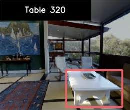
Under review as a conference paper at ICLR 2021
    A) Instance Category Distribution             B) Frames Between Occurrences   C) Unique Viewpoints / 100 Frames

Figure 3: Statistics for our RoamingRooms dataset. Plots show a natural long tail distribution of
instances grouped into categories. An average sequence has 3 different view points. Sequences are
highly correlated in time but revisits are not uncommon.

context as a cue, forgetting occurs. Our proposed CPM contains parallels to human brain memory
components (Cohen & Squire, 1980). Long term statistical learning is captured in a CNN that
produces a deep embedding. An RNN holds a type of working memory that can retain novel objects
and spatiotemporal contexts. Lastly, the prototype memory represents the semantic memory, which
consolidates multiple events into a single knowledge vector (Duff et al., 2020). Other deep learning
researchers have proposed multiple memory systems for continual learning. In Parisi et al. (2018),
the learning algorithm is heuristic and representations come from pretrained networks. In Kemker
& Kanan (2018), a prototype memory is used for recalling recent examples and rehearsal from a
generative model allows this knowledge to be integrated and distilled into a long-term memory.

3      O NLINE C ONTEXTUALIZED F EW-S HOT L EARNING
In this section, we introduce our new online contextualized few-shot learning (OC-FSL) setup in the
form of a sequential decision problem, and then introduce our new benchmark datasets.
Continual few-shot classification as a sequential decision problem: In traditional few-shot learn-
ing, an episode is constructed by a support set S and a query set Q. A few-shot learner f is expected
to predict the class of each example in the query set xQ based on the support set information:
ŷ Q = f (xQ ; (xS1 , y1S ), . . . , (xSN , yN
                                             S
                                               )), where x ∈ RD , and y ∈ [1 . . . K]. This setup is not a natural
fit for continual learning, since it is unclear when to insert a query set into the sequence.
Inspired by the online learning literature, we can convert continual few-shot learning into a se-
quential decision problem, where every input example is also part of the evaluation: ŷt =
f (xt ; (x1 , ỹ1 ), . . . , (xt−1 , ỹt−1 )), for t = 1 . . . T , where ỹ here further allows that the sequence
of inputs to be semi-supervised: ỹ equals yt if labeled, or otherwise −1. The setup in Santoro et al.
(2016) and Kaiser et al. (2017) is similar; they train RNNs using such a temporal sequence as input.
However, their evaluation relies on a “query set” at the end. We instead evaluate online while learning.
Figure 1-A illustrates these features, using an example of an input sequence where an agent is learning
about new objects in a kitchen. The model is rewarded when it correctly predicts a known class or
when it indicates that the item has yet to be assigned a label.
Contextualized environments: Typical continual learning consists of a sequence of tasks, and
models are trained sequentially for each task. This feature is also preserved in many incremental
learning settings (Rebuffi et al., 2017). For instance, the split-CIFAR task divides CIFAR-100 into 10
learning environments, each with 10 classes, presented sequentially. In our formulation, the sequence
returns to earlier environments (see Figure 1-B), which enables assessment of long-term durability
of knowledge. Although the ground-truth environment identity is not provided, we structure the
task such that the environment itself provides contextual cues which can constrain the correct class
label. Spatial cues in the input help distinguish one environment from another. Temporal cues are
implicit because the sequence tends to switch environments infrequently, allowing recent inputs to be
beneficial in guiding the interpretation of the current input.
RoamingOmniglot: The Omniglot dataset (Lake et al., 2015) contains 1623 handwritten characters
from 50 different alphabets. We split the alphabets into 31 for training, 5 for validation, and 13
for testing. We augment classes by 90 degree rotations to create 6492 classes in total. Each
contextualized few-shot learning image sequence contains 150 images, drawn from a random sample
of 5-10 alphabets, for a total of 50 classes per sequence. These classes are randomly assigned
to 5 different environments; within an environment, the characters are distributed according to a
Chinese restaurant process (Aldous, 1985) to mimic the imbalanced long-tail distribution of naturally
occurring objects. We switch between environments using a Markov switching process; i.e., at each
step there is a constant probability of switching to another environment. An example sequence is
shown in Figure 2-A.

                                                        4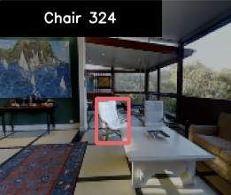
Under review as a conference paper at ICLR 2021

    Contextual RNN                      Context Vector
                                        & Control
                                                                                       Figure 4: Contextual prototypical memory.
    …      RNN       RNN   RNN
                                   +
                                        Param.
                                                            Cls 1
                                                                                       Temporal contextual features are extracted from an
                                                                              Cls 2

                                                                                       RNN. The prototype memory stores one vector per
    …      CNN       CNN   CNN                     Online Avg.                         class and does online averaging. Examples falling
                                                                    Cls 3
                                                                    Prototype Memory   outside the radii of all prototypes are classified as
                                 time
            t-2      t-1    t
                                                                                       “new.”

RoamingRooms: As none of the current few-shot learning datasets provides the natural online
learning experience that we would like to study, we created our own dataset using simulated indoor
environments. We formulate this as a few-shot instance learning problem, which could be a use case
for a home robot: it needs to quickly recognize and differentiate novel object instances, and large
viewpoint variations can make this task challenging (see examples in Figure 2-B). There are over
7,000 unique instance classes in the dataset, making it suitable to meta-learning approaches.
Our dataset is derived from the Matterport3D dataset (Chang et al., 2017), which has 90 indoor
worlds captured using panoramic depth cameras. We split these into 60 worlds for training, 10 for
validation and 20 for testing. We use MatterSim (Anderson et al., 2018) to load the simulated world
and collect camera images and use HabitatSim (Savva et al., 2019) to simulate 3D mesh and align
instance segmentation labels onto 2D image space. We created a random walking agent to collect the
virtual visual experience. For each viewpoint in the random walk, we randomly sample one object
from the image sensor and highlight it with the available instance segmentation, forming an input
frame. Each viewpoint provides environmental context—the other objects present in the room with
the highlighted object.
Figure 3-A shows the object instance distribution. We see strong temporal correlation, as 30% of
the time the same instance appears in the next frame (Figure 3-B), but there is also a significant
proportion of revisits. On average, there are three different viewpoints per 100-image sequence
(Figure 3-C). Details and other statistics of our proposed datasets are included in the Appendix.

4       C ONTEXTUAL P ROTOTYPICAL M EMORY N ETWORKS
In the online contextualized few-shot learning setup, the few-shot learner can potentially improve
by modeling the temporal context. Metric learning approaches (Snell et al., 2017) typically ignore
temporal contextual relations and directly compare the similarity between training and test samples.
Gradient-based approaches (Javed & White, 2019), on the other hand, have the ability to adapt to new
contexts, but they do not naturally handle new and unlabeled examples. Inspired by the contextual
binding theory of human memory (Yonelinas et al., 2019), we propose a simple yet effective approach
that uses an RNN to transmit spatiotemporal context and control signals to a prototype memory
(Figure 4).
Prototype memory: We start describing our model with the prototype memory, which is an online
version of the Prototypical Network (or ProtoNet) (Snell et al., 2017). ProtoNet can be viewed as
a knowledge base memory, where each object class k is represented by a prototype vector p[k],
computed as the mean vector of all the support instances of the class in a sequence. It can also be
applied to our task of online few-shot learning naturally, with some modifications. Suppose that at
time-step t we have already stored a few classes in the memory, each represented by their current
prototype pt [k], and we would like to query the memory using the input feature ht . We model
our prototype memory as ŷt,k = softmax(−dmt (ht , pt [k])), (e.g. squared Euclidean distance or
cosine dissimilarity) parameterized by a vector mt that scales each dimension with a Hadamard
product. To predict whether an example is of a new class, we can use a separate novelty output ûrt
with sigmoid activation, similar to the approach introduced in Ren et al. (2018), where βtr and γtr are
yet-to-be-specified thresholding hyperparameters (the superscript r stands for read):
                                            ûrt = σ((min dmt (ht , pt [k]) − βtr )/γtr ).                                             (1)
                                                                       k
Memory consolidation with online prototype averaging: Traditionally, ProtoNet uses the aver-
age representation of a class across all support examples. Here, we must be able to adapt the prototype
memory incrementally at each step. Fortunately, we can recover the computation of a ProtoNet by
performing a simple online averaging:
                                                            1
                      ct = ct−1 + 1; A(ht ; pt−1 , ct ) = (pt−1 ct−1 + ht ) ,                        (2)
                                                            ct
where h is the input feature, and p is the prototype, and c is a scalar indicating the number of
examples that have been added to this prototype up to time t. The online averaging function A can
also be made more flexible to allow more plasiticity, modeled by a gated averaging unit (GAU):

                                                                                       5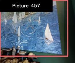
Under review as a conference paper at ICLR 2021

Table 1: RoamingOmniglot OC-FSL results. Max 5 env, 150 images, 50 cls, with 8×8 occlusion.
                                            Supervised                            Semi-supervised
                Method
                               AP       1-shot Acc.    3-shot Acc.       AP      1-shot Acc.    3-shot Acc.
                 LSTM        64.34     61.00 ± 0.22     81.85 ± 0.21    54.34   68.30 ± 0.20   76.38 ± 0.49
                  DNC        81.30     78.87 ± 0.19     91.01 ± 0.15    81.37   88.56 ± 0.12   93.81 ± 0.26
                OML-U        77.38     70.98 ± 0.21     89.13 ± 0.16    66.70   74.65 ± 0.19   90.81 ± 0.34
               OML-U++       86.85     88.43 ± 0.14     92.01 ± 0.14    81.39   71.64 ± 0.19   93.72 ± 0.27
                 O-MN        88.69     84.82 ± 0.15     95.55 ± 0.11    84.39   88.77 ± 0.13   97.28 ± 0.17
                 O-IMP       90.15     85.74 ± 0.15     96.66 ± 0.09    81.62   88.68 ± 0.13   97.09 ± 0.19
                 O-PN        90.49     85.68 ± 0.15     96.95 ± 0.09    84.61   88.71 ± 0.13   97.61 ± 0.17
               CPM (Ours)    94.17     91.99 ± 0.11     97.74 ± 0.08    90.42   93.18 ± 0.16   97.89 ± 0.15

            Table 2: RoamingRooms OC-FSL results. Max 100 images and 40 classes.
                                            Supervised                           Semi-supervised
                Method
                              AP        1-shot Acc.    3-shot Acc.       AP     1-shot Acc.    3-shot Acc.
                LSTM         45.67     59.90 ± 0.40     61.85 ± 0.45    33.32   52.71 ± 0.38   55.83 ± 0.76
                 DNC         80.86     82.15 ± 0.32     87.30 ± 0.30    73.49   80.27 ± 0.33   87.87 ± 0.49
               OML-U         76.27     73.91 ± 0.37     83.99 ± 0.33    63.40   70.67 ± 0.38   85.25 ± 0.56
              OML-U++        88.03     88.32 ± 0.27     89.61 ± 0.29    81.90   84.79 ± 0.31   89.80 ± 0.47
                O-MN         85.91     82.82 ± 0.32     89.99 ± 0.26    78.99   80.08 ± 0.34   92.43 ± 0.41
                O-IMP        87.33     85.28 ± 0.31     90.83 ± 0.25    75.36   84.57 ± 0.31   91.17 ± 0.43
                O-PN         86.01     84.89 ± 0.31     89.58 ± 0.28    76.36   80.67 ± 0.34   88.83 ± 0.49
              CPM (Ours)     89.14     88.39 ± 0.27     91.31 ± 0.26    84.12   86.17 ± 0.30   91.16 ± 0.44

      AGAU (ht ; pt−1 ) = (1 − ft ) · pt−1 + ft · ht , where ft = σ(Wf [ht , pt−1 ] + bf ) ∈ R.      (3)
When the current example is unlabeled, yt is encoded as −1, and the model’s own prediction ŷt will
determine which prototype to update; in this case, the model must also determine a strength of belief,
ûw                                                                                w
  t , that the current unlabeled example should be treated as a new class. Given ût and ŷt , the model
can then update a prototype:
               ûw                               w    w
                 t = σ((min dmt (ht , pt [k]) − βt )/γt ),                                                              (4)
                              k
            ∆[k]t = 1[yt = k] + ŷt,k (1 −            ûw
                                                        t )1[yt = −1],                                                  (5)
                    | {z } |                             {z             }
                         Supervised                Unsupervised

             c[k]t = c[k]t−1 + ∆[k]t ,                                                                                  (6)
             p[k]t = A(ht ∆[k]t ; p[k]t−1 , c[k]t ), or p[k]t = AGAU (ht ∆[k]t ; p[k]t−1 ).                             (7)
As-yet-unspecified hyperparameters βtw and γtw are required (the superscript w is for write). These
parameters for the online-updating novelty output ûw                        r      r
                                                       t are distinct from βt and γt in Equation 1. The
intuition is that for “self-teaching” to work, the model potentially needs to be more conservative in cre-
ating new classes (avoiding corruption of prototypes) than in predicting an input as being a new class.
Contextual RNN: Instead of directly using the features from the CNN hCNN          t   as input features to
the prototype memory, we would also like to use contextual information from the recent past. Above
we introduced threshold hyperparameters βtr , γtr , βtw , γtw as well as the metric parameter Mt . We let
the contextual RNN output these additional control parameters, so that the unknown thresholds and
metric function can adapt based on the information in the context. The RNN produces the context
vector hRNN
         t   and other control parameters conditioned on hCNN   t   :
                                       r    r     w      w
                       zt , ht , mt , βt , γt , βt , γt = RNN(hCNN
                             RNN

                                                                        t   ; zt−1 ),                  (8)
where zt is the recurrent state of the RNN, and mt is the scaling factor in the dissimilarity score.
The context, hRNN
               t   , serves as an additive bias on the state vector used for FSL: ht = hCNN
                                                                                        t   + hRNN
                                                                                                t  .
This addition operation in the feature space can help contextualize prototypes based on temporal
proximity, and is also similar to how the human brain leverages spatiotemporal context for memory
storage (Yonelinas et al., 2019).
Loss function: The loss function is computed after an entire sequence ends and all network
parameters are learned end-to-end. The loss is composed of two parts. The first is binary cross-
entropy (BCE), for telling whether each example has been assigned a label or not, i.e., prediction of
new classes. Second we use a multi-class cross-entropy for classifying among the known ones. We
can write down the overall loss function as follows:
            T                                                         K
         1X
              λ [−1[yt < 0] log(ûrt ) − 1[yt ≥ 0] log(1 − ûrt )] +     −1[yt = k] log(ŷt,k ) .
                                                                     X
    L=                                                                                                                  (9)
         T t=1 |                        {z                       }       |       {z          }
                                                                     k=1
                                  Binary cross entropy on old vs. new                    Cross entropy on old classes

                                                               6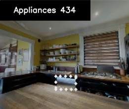
Under review as a conference paper at ICLR 2021
                                   RoamingOmniglot (Sup.)               RoamingOmniglot (Semi-Sup.)                                    RoamingRooms (Sup.)                RoamingRooms (Semi-Sup.)
      100                                               100                                              100                                            100
                                                                                                          95                                             95
       95                                                95                                               90                                             90
                 Offline LR                                                                                          Offline LR

Acc

                                                  Acc

                                                                                                   Acc

                                                                                                                                                  Acc
       90        DNC                                     90                                               85         DNC                                 85
                 OML-U++                                                                                  80         OML-U++                             80
       85        Online PN                               85                                                          Online PN
                 CPM (Ours)                                                                               75         CPM (Ours)                          75
       80                                             80                                                  70                                             70
            0    20    40     60      80    100    120 0      20   40     60      80   100   120               0        20        40      60      80          0     20    40      60      80
                              Time                                         Time                                                    Time                                    Time
Figure 5: Few-shot classification accuracy over time. Left: RoamingOmniglot. Right: Roamin-
gRooms. Top: Supervised. Bottom: Semi-supervised. An offline logistic regression (Offline LR)
baseline is also included, using pretrained ProtoNet features. It is trained on all labeled examples
except for the one at the current time step.
                                                                                                                                                                          95
                                                                                                                                  Online PN         CPM (Ours)

                                                                                                                                                                          90

                                                                                                                                                                           AP
                                                                                                                                                                          85

                                                                                                                                                                          80
                                                                                                                   No Context     +Temporal     +Spatial          +Both
Figure 6: Effect of spatiotemporal context. Spatiotemporal context are added separately and
together in RoamingOmniglot, by introducing texture background and temporal correlation. Left:
Stimuli used for spatial cue of the background environment. Right: Our CPM model benefits from
the presence of a temporal context (“+Temporal” and “+Both”)

5               E XPERIMENTS
In this section, we show experimental results for our online contextualized few-shot learning paradigm,
using RoamingOmniglot and RoamingRooms (see Sec. 3) to evaluate our model, CPM, and other
state-of-the-art methods. For Omniglot, we apply an 8×8 CutOut (Devries & Taylor, 2017) to each
image to make the task more challenging.
Implementation details: For the RoamingOmniglot experiment we used the common 4-layer CNN
for few-shot learning with 64 channels in each layer. For the RoamingRooms experiment we resize
the input to 120×160 and we use the ResNet-12 architecture (Oreshkin et al., 2018). To represent the
feature of the input image with an attention mask, we concatenate the global average pooled feature
with the attention ROI feature, resulting in a 512d feature vector. For the contextual RNN, in both
experiments we used an LSTM (Hochreiter & Schmidhuber, 1997) with a 256d hidden state. The
best CPM model is equipped using GAU and cosine similarity for querying prototypes. Logits based
on cosine similarity are multiplied with a learned scalar initialized at 10.0 (Oreshkin et al., 2018). We
include additional training details in Appendix B.
Evaluation metrics: In order to compute a single number that characterizes the learning ability
over sequences, we propose to use average precision (AP) to combine the prediction on old and
new classes. Concretely, all predictions are sorted by their old vs. new scores, and we compute AP
using the area under the precision-recall curve. True positive is defined as the correct prediction of a
multi-class classification among known classes. We also compute the “N -shot” accuracy; i.e., the
average accuracy after seeing the label N times in the sequence. Note that these accuracy scores only
reflect the performance on known class predictions. All numbers are reported with an average over
2,000 sequences and for N -shot accuracy standard error is also included.
Comparisons: To evaluate the merits of our proposed model, we implement classic few-shot
learning and online meta-learning methods. More implementation and training details of these
baseline methods can be found in Appendix B.
• OML (Javed & White, 2019): This is an online version of MAML (Finn et al., 2017). It performs
  one gradient descent step for each labeled input image, and slow weights are learned via back-
  propagation through time. On top of OML, we added an unknown predictor ût = 1 − maxk ŷt,k 1
  (OML-U). We also found that using cosine classifier without the last layer ReLU is much better
  than using the original dot-product classifier, and this improvement is denoted as OML-U++.
• LSTM (Hochreiter & Schmidhuber, 1997) & DNC (Graves et al., 2016): We include RNN methods
  for comparison as well. Differentiable neural computer (DNC) is an improved version of memory
  augmented neural network (MANN) (Santoro et al., 2016).
• Online MatchingNet (O-MN) (Vinyals et al., 2016), IMP (O-IMP) (Allen et al., 2019) & Pro-
  toNet (O-PN) (Snell et al., 2017): We used the same negative Euclidean distance as the similarity
        1
            We tried a few other ways and this is found to be the best.

                                                                                                   7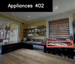
Under review as a conference paper at ICLR 2021

Table 3: Ablation of CPM architectural com-                             Table 4: Ablation of semi-supervised learning
ponents on RoamingOmniglot                                              components on RoamingOmniglot
        Method        hRNN   βt∗ , γt∗   Metric mt   GAU   Val AP         Method   RNN   Prototype   βtw , γtw   GAU   Val AP
         O-PN                                              91.22
                                                                          O-PN                                         90.83
       No hRNN                  3           3              92.52
       hRNN only       3                                   93.48          O-PN              3                          89.10
     No metric mt      3        3                          93.61          O-PN              3           3              91.22
       No βt∗ , γt∗    3                    3              93.98          CPM                                          92.57
      ht = hRNNt       3        3           3              93.70          CPM      3                                   93.16
     CPM Avg. Euc      3        3           3              94.08          CPM      3        3                          93.20
     CPM Avg. Cos      3        3           3              94.57
     CPM GAU Euc       3        3           3        3     94.11          CPM      3        3           3              94.08
     CPM GAU Cos       3        3           3        3     94.65          CPM      3        3           3        3     94.65

    function for these three metric learning based approaches. In particular, MatchingNet stores all
    examples and performs nearest neighbor matching, which can be memory inefficient. Note that
    Online ProtoNet is a variant of our method without the contextual RNN.

Main results: Our main results are shown in Table 1 and 2, including both supervised and semi-
supervised settings. Our approach achieves the best performance on AP consistently across all
settings. Online ProtoNet is a direct comparison without our contextual RNN and it is clear that CPM
is significantly better. Our method is slightly worse than Online MatchingNet in terms of 3-shot
accuracy on the RoamingRooms semisupervised benchmark. This can be explained by the fact that
MatchingNet stores all past seen examples, whereas CPM only stores one prototype per class. Per
timestep accuracy is plotted in Figure 5, and the decaying accuracy is due to the increasing number
of classes over time. In RoamingOmniglot, CPM is able to closely match or even sometimes surpass
the offline classifier, which re-trains at each step and uses all images in a sequence except the current
one. This is reasonable as our model is able to leverage information from the current context.

Effect of spatiotemporal context: To answer the question whether the gain in performance is
due to spatiotemporal reasoning, we conduct the following experiment comparing CPM with online
ProtoNet. We allow the CNN to have the ability to recognize the context in RoamingOmniglot by
adding a texture background image using the Kylberg texture dataset (Kylberg, 2011) (see Figure 6
left). As a control, we can also destroy the temporal context by shuffling all the images in a sequence.
We train four different models on dataset controls with or without the presence of spatial or temporal
context, and results are shown in Figure 6. First, both online ProtoNet and CPM benefit from the
inclusion of a spatial context. This is understandable as the CNN has the ability to learn spatial cues,
which re-confirms our main hypothesis that successful inference of the current context is beneficial
to novel object recognition. Second, only our CPM model benefits from the presence of temporal
context, and it receives distinct gains from spatial and temporal contexts.

Ablation studies: We ablate each individual module we introduce. Results are shown in Tables 3
and 4. Table 3 studies different ways we use the RNN, including the context vector hRNN , the predicted
threshold parameters βt∗ , γt∗ , and the predicted metric scaling vector t . Table 4 studies various ways
to learn from unlabeled examples, where we separately disable the RNN update, prototype update,
and distinct write-threshold parameters βtw , γtw (vs. using read-threshold parameters), which makes
it robust to potential mistakes made in semi-supervised learning. We verify that each component has
a positive impact on the performance.

6     C ONCLUSION
We proposed online contextualized few-shot learning, OC-FSL, a paradigm for machine learning
that emulates a human or artificial agent interacting with a physical world. It combines multiple
properties to create a challenging learning task: every input must be classified or flagged as novel,
every input is also used for training, semi-supervised learning can potentially improve performance,
and the temporal distribution of inputs is non-IID and comes from a generative model in which input
and class distributions are conditional on a latent environment with Markovian transition probabilities.
We proposed the RoamingRooms dataset to simulate an agent wandering within a physical world.
We also proposed a new model, CPM, which uses an RNN to extract spatiotemporal context from
the input stream and to provide control settings to a prototype-based FSL model. In the context of
naturalistic domains like RoamingRooms, CPM is able to leverage contextual information to attain
performance unmatched by other state-of-the-art FSL methods.

                                                                    8
Under review as a conference paper at ICLR 2021
R EFERENCES
David J Aldous. Exchangeability and related topics. In École d’Été de Probabilités de Saint-Flour
XIII—1983, pp. 1–198. Springer, 1985.
Kelsey R. Allen, Evan Shelhamer, Hanul Shin, and Joshua B. Tenenbaum. Infinite mixture prototypes
for few-shot learning. In Proceedings of the 36th International Conference on Machine Learning,
ICML, 2019.
Peter Anderson, Qi Wu, Damien Teney, Jake Bruce, Mark Johnson, Niko Sünderhauf, Ian Reid,
Stephen Gould, and Anton van den Hengel. Vision-and-Language Navigation: Interpreting visually-
grounded navigation instructions in real environments. In Proceedings of the IEEE Conference on
Computer Vision and Pattern Recognition, CVPR, 2018.
Antreas Antoniou, Massimiliano Patacchiola, Mateusz Ochal, and Amos J. Storkey. Defining
benchmarks for continual few-shot learning. CoRR, abs/2004.11967, 2020.
Massimo Caccia, Pau Rodríguez, Oleksiy Ostapenko, Fabrice Normandin, Min Lin, Lucas Caccia,
Issam H. Laradji, Irina Rish, Alexandre Lacoste, David Vázquez, and Laurent Charlin. Online
fast adaptation and knowledge accumulation: a new approach to continual learning. CoRR,
abs/2003.05856, 2020.
Francisco M. Castro, Manuel J. Marín-Jiménez, Nicolás Guil, Cordelia Schmid, and Karteek Alahari.
End-to-end incremental learning. In 15th European Conference on Computer Vision, ECCV, 2018.
Angel X. Chang, Angela Dai, Thomas A. Funkhouser, Maciej Halber, Matthias Nießner, Manolis
Savva, Shuran Song, Andy Zeng, and Yinda Zhang. Matterport3d: Learning from RGB-D data in
indoor environments. In International Conference on 3D Vision, 3DV, 2017.
NJ Cohen and LR Squire. Preserved learning and retention of pattern-analyzing skill in amnesia:
dissociation of knowing how and knowing that. Science, 210(4466):207–210, 1980. ISSN
0036-8075. doi: 10.1126/science.7414331.
Terrance Devries and Graham W. Taylor. Improved regularization of convolutional neural networks
with cutout. CoRR, abs/1708.04552, 2017.
Melissa C. Duff, Natalie V. Covington, Caitlin Hilverman, and Neal J. Cohen. Semantic mem-
ory and the hippocampus: Revisiting, reaffirming, and extending the reach of their critical
relationship. Frontiers in Human Neuroscience, 13:471, 2020. ISSN 1662-5161. doi: 10.
3389/fnhum.2019.00471. URL https://www.frontiersin.org/article/10.3389/
fnhum.2019.00471.
Chelsea Finn, Pieter Abbeel, and Sergey Levine. Model-agnostic meta-learning for fast adaptation of
deep networks. In Proceedings of the 34th International Conference on Machine Learning, ICML,
2017.
Chelsea Finn, Aravind Rajeswaran, Sham M. Kakade, and Sergey Levine. Online meta-learning. In
Proceedings of the 36th International Conference on Machine Learning, ICML, 2019.
Spyros Gidaris and Nikos Komodakis. Dynamic few-shot visual learning without forgetting. In IEEE
Conference on Computer Vision and Pattern Recognition, CVPR, 2018.
Alex Graves, Greg Wayne, Malcolm Reynolds, Tim Harley, Ivo Danihelka, Agnieszka Grabska-
Barwińska, Sergio Gómez Colmenarejo, Edward Grefenstette, Tiago Ramalho, John Agapiou,
Adrià Puigdomènech Badia, Karl Moritz Hermann, Yori Zwols, Georg Ostrovski, Adam Cain,
Helen King, Christopher Summerfield, Phil Blunsom, Koray Kavukcuoglu, and Demis Hassabis.
Hybrid computing using a neural network with dynamic external memory. Nature, 538(7626):
471–476, Oct 2016. ISSN 1476-4687. doi: 10.1038/nature20101.
James Harrison, Apoorva Sharma, Chelsea Finn, and Marco Pavone. Continuous meta-learning
without tasks. CoRR, abs/1912.08866, 2019.
Jiangpeng He, Runyu Mao, Zeman Shao, and Fengqing Zhu. Incremental learning in online scenario.
In IEEE/CVF Conference on Computer Vision and Pattern Recognition, CVPR, 2020.
9Under review as a conference paper at ICLR 2021
Sepp Hochreiter and Jürgen Schmidhuber. Long short-term memory. Neural Comput., 9(8):
1735–1780, nov 1997. ISSN 0899-7667. doi: 10.1162/neco.1997.9.8.1735.
Saihui Hou, Xinyu Pan, Chen Change Loy, Zilei Wang, and Dahua Lin. Learning a unified classifier
incrementally via rebalancing. In IEEE Conference on Computer Vision and Pattern Recognition,
CVPR, 2019.
M. W. Howard. Temporal and spatial context in the mind and brain. Current opinion in behavioral
sciences, 17:14–19, 2017.
Khurram Javed and Martha White. Meta-learning representations for continual learning. In Ad-
vances in Neural Information Processing Systems 32: Annual Conference on Neural Information
Processing Systems, NeurIPS, 2019.
Ghassen Jerfel, Erin Grant, Tom Griffiths, and Katherine A. Heller. Reconciling meta-learning and
continual learning with online mixtures of tasks. In Advances in Neural Information Processing
Systems 32: Annual Conference on Neural Information Processing Systems, NeurIPS, 2019.
Michael J. Kahana. Foundations of human memory. Oxford University Press, New York, 2012. ISBN
9780195333244. OCLC: ocn744297060.
Lukasz Kaiser, Ofir Nachum, Aurko Roy, and Samy Bengio. Learning to remember rare events. In
5th International Conference on Learning Representations, ICLR, 2017.
Ronald Kemker and Christopher Kanan. Fearnet: Brain-inspired model for incremental learning. In
Proceedings of 6th International Conference on Learning Representations (ICLR), 2018.
Diederik P. Kingma and Jimmy Ba. Adam: A method for stochastic optimization. In 3rd International
Conference on Learning Representations, ICLR, 2015.
James Kirkpatrick, Razvan Pascanu, Neil Rabinowitz, Joel Veness, Guillaume Desjardins, Andrei A.
Rusu, Kieran Milan, John Quan, Tiago Ramalho, Agnieszka Grabska-Barwinska, Demis Hassabis,
Claudia Clopath, Dharshan Kumaran, and Raia Hadsell. Overcoming catastrophic forgetting in
neural networks. Proceedings of the National Academy of Sciences, 114(13):3521–3526, 2017.
Gregory Koch, Richard Zemel, and Ruslan Salakhutdinov. Siamese neural networks for one-shot
image recognition. In ICML deep learning workshop, volume 2, 2015.
Alex Krizhevsky. Learning multiple layers of features from tiny images. Technical report, University
of Toronto, 2009.
Gustaf Kylberg. Kylberg Texture Dataset v. 1.0. Centre for Image Analysis, Swedish University of
Agricultural Sciences and . . . , 2011.
Brenden M Lake, Ruslan Salakhutdinov, and Joshua B Tenenbaum. Human-level concept learning
through probabilistic program induction. Science, 350(6266):1332–1338, 2015.
Y. Lecun, L. Bottou, Y. Bengio, and P. Haffner. Gradient-based learning applied to document
recognition. Proceedings of the IEEE, 86(11):2278–2324, Nov 1998. ISSN 0018-9219. doi:
10.1109/5.726791.
Fei-Fei Li, Robert Fergus, and Pietro Perona. Learning generative visual models from few training
examples: An incremental bayesian approach tested on 101 object categories. Comput. Vis. Image
Underst., 106(1):59–70, 2007.
Zhenguo Li, Fengwei Zhou, Fei Chen, and Hang Li. Meta-sgd: Learning to learn quickly for few
shot learning. CoRR, abs/1707.09835, 2017.
Zhizhong Li and Derek Hoiem. Learning without forgetting. IEEE Trans. Pattern Anal. Mach. Intell.,
40(12):2935–2947, 2018.
Vincenzo Lomonaco and Davide Maltoni. Core50: a new dataset and benchmark for continuous
object recognition. In 1st Annual Conference on Robot Learning, CoRL, 2017.
10Under review as a conference paper at ICLR 2021
David Lopez-Paz and Marc’Aurelio Ranzato. Gradient episodic memory for continual learning. In
Advances in Neural Information Processing Systems 30: Annual Conference on Neural Information
Processing Systems, NeurIPS, 2017.
Laurens van der Maaten and Geoffrey Hinton. Visualizing data using t-sne. Journal of machine
learning research, 9(Nov):2579–2605, 2008.
James McClelland, Bruce McNaughton, and Randall O’Reilly. Why there are complementary
learning systems in the hippocampus and neocortex: Insights from the successes and failures of
connectionist models of learning and memory. Psychological review, 102:419–57, 08 1995. doi:
10.1037/0033-295X.102.3.419.
Michael McCloskey and Neal J Cohen. Catastrophic interference in connectionist networks: The
sequential learning problem. In Psychology of learning and motivation, volume 24, pp. 109–165.
Elsevier, 1989.
Marius Muja and David Lowe. Flann-fast library for approximate nearest neighbors user manual.
Computer Science Department, University of British Columbia, Vancouver, BC, Canada, 2009.
Boris N. Oreshkin, Pau Rodríguez López, and Alexandre Lacoste. TADAM: task dependent adaptive
metric for improved few-shot learning. In Advances in Neural Information Processing Systems 31:
Annual Conference on Neural Information Processing Systems, NeurIPS, 2018.
German I. Parisi, Jun Tani, Cornelius Weber, and Stefan Wermter. Lifelong learning of spatiotemporal
representations with dual-memory recurrent self-organization. Frontiers in neurorobotics, 12:
78–78, Nov 2018. ISSN 1662-5218. doi: 10.3389/fnbot.2018.00078.
Sylvestre-Alvise Rebuffi, Alexander Kolesnikov, Georg Sperl, and Christoph H. Lampert. icarl:
Incremental classifier and representation learning. In IEEE Conference on Computer Vision and
Pattern Recognition, CVPR, 2017.
Mengye Ren, Eleni Triantafillou, Sachin Ravi, Jake Snell, Kevin Swersky, Joshua B. Tenenbaum,
Hugo Larochelle, and Richard S. Zemel. Meta-learning for semi-supervised few-shot classification.
In 6th International Conference on Learning Representations, ICLR, 2018.
Mengye Ren, Renjie Liao, Ethan Fetaya, and Richard S. Zemel. Incremental few-shot learning with
attention attractor networks. In Advances in Neural Information Processing Systems 32: Annual
Conference on Neural Information Processing Systems, NeurIPS, 2019.
Adam Santoro, Sergey Bartunov, Matthew Botvinick, Daan Wierstra, and Timothy P. Lillicrap.
Meta-learning with memory-augmented neural networks. In Proceedings of the 33nd International
Conference on Machine Learning, ICML, 2016.
Manolis Savva, Abhishek Kadian, Oleksandr Maksymets, Yili Zhao, Erik Wijmans, Bhavana Jain,
Julian Straub, Jia Liu, Vladlen Koltun, Jitendra Malik, Devi Parikh, and Dhruv Batra. Habitat: A
Platform for Embodied AI Research. In Proceedings of the IEEE/CVF International Conference
on Computer Vision, ICCV, 2019.
Jürgen Schmidhuber. Evolutionary principles in self-referential learning, or on learning how to learn:
The meta-meta-... hook. Diplomarbeit, Technische Universität München, München, 1987.
Qi She, Fan Feng, Xinyue Hao, Qihan Yang, Chuanlin Lan, Vincenzo Lomonaco, Xuesong Shi,
Zhengwei Wang, Yao Guo, Yimin Zhang, Fei Qiao, and Rosa H. M. Chan. Openloris-object: A
dataset and benchmark towards lifelong object recognition. CoRR, abs/1911.06487, 2019.
Jake Snell, Kevin Swersky, and Richard S. Zemel. Prototypical networks for few-shot learning. In
Advances in Neural Information Processing Systems 30: Annual Conference on Neural Information
Processing Systems, NeurIPS, 2017.
Xiaoyu Tao, Xiaopeng Hong, Xinyuan Chang, Songlin Dong, Xing Wei, and Yihong Gong. Few-shot
class-incremental learning. CoRR, abs/2004.10956, 2020.
Sebastian Thrun. Lifelong learning algorithms. In Learning to learn, pp. 181–209. Springer, 1998.
11Under review as a conference paper at ICLR 2021
Oriol Vinyals, Charles Blundell, Tim Lillicrap, Koray Kavukcuoglu, and Daan Wierstra. Matching
networks for one shot learning. In Advances in Neural Information Processing Systems 29: Annual
Conference on Neural Information Processing Systems, NeurIPS, 2016.
Yue Wu, Yinpeng Chen, Lijuan Wang, Yuancheng Ye, Zicheng Liu, Yandong Guo, and Yun Fu. Large
scale incremental learning. In IEEE Conference on Computer Vision and Pattern Recognition,
CVPR, 2019.
Andrew P. Yonelinas, Charan Ranganath, Arne D. Ekstrom, and Brian J. Wiltgen. A contextual bind-
ing theory of episodic memory: systems consolidation reconsidered. Nature reviews. Neuroscience,
20(6):364–375, Jun 2019. ISSN 1471-0048. doi: 10.1038/s41583-019-0150-4.
Jaehong Yoon, Eunho Yang, Jeongtae Lee, and Sung Ju Hwang. Lifelong learning with dynamically
expandable networks. In 6th International Conference on Learning Representations, ICLR, 2018.
12Under review as a conference paper at ICLR 2021
A DATASET D ETAILS
A.1 B ENCHMARK COMPARISON
We include Table 6 to compare existing continual and few-shot learning paradigms.
A.2 ROAMING O MNIGLOT D ETAILS
For the RoamingOmniglot experiments, we use sequences with maximum 150 images, from 5
environments. For individual environment, we use a Chinese restaurant process to sample the class
distribution. In particular, the probability of sampling a new class is:
kα + θ
pnew = , (10)
m+θ
where k is the number of classes that we have already sampled in the environment, and m is the total
number of instances we have in the environment. α is set to 0.2 and θ is set to 1.0 in all experiments.
The environment switching is implemented by a Markov switching process. At each step in the
sequence there is a constant probability pswitch that switches to another environment. For all experi-
ments, we set pswitch to 0.2. We truncate the maximum number of appearances per class to 6. If the
maximum appearance is reached, we will sample another class.
A.3 A DDITIONAL ROAMING ROOMS S TATISTICS
Statistics of the RoamingRooms are included in Table 5, in comparison to other few-shot and continual
learning datasets. Note that since RoamingRooms is collected from a simulated environment, with 90
indoor worlds consisting of 1.2K panorama images and 1.22M video frames. The dataset contains
about 6.9K random walk sequences with a maximum of 200 frames per sequence. For training we
randomly crop 100 frames to form a training sequence. There are 7.0K unique instance classes.
Plots of additional statistics of RoamingRooms are shown in Figure 7. In addition to the ones shown
in the main paper, instances and viewpoints also follow long tail distributions. The number of objects
in each frame follows an exponential distribution.
A.4 ROAMING ROOMS S IMULATOR D ETAILS
We generate our episodes with a two-stage process using two simulators – HabitatSim (Savva et al.,
2019) and MatterSim (Anderson et al., 2018) – because HabitatSim is based on 3D meshes and using
HabitatSim alone will result in poor image quality due to incorrect mesh reconstruction. Therefore we
sacrificed the continuous movement of agents within HabitatSim and base our environment navigation
on the discrete viewpoints in MatterSim, which is based on real panoramic images. The horizontal
field of view is set to 90 degrees for HabitatSim and 100 degrees for MatterSim, and we simulate
with 800×600 resolution.
The first stage of generation involves randomly picking a sequence of viewpoints on the connectivity
graph within MatterSim. For each viewpoint, the agent scans the environment along the yaw and
pitch axes for a random period of time until a navigable viewpoint is within view. The time spent
in a single viewpoint follows a Gaussian distribution with mean 5.0 and standard deviation 1.0. At
the start of each new viewpoint, the agent randomly picks a direction to rotate and takes 12.5 degree
steps along the yaw axis, and with 95% probability, a 5 degree rotation along the pitch axis is applied
in a randomly chosen direction. When a navigable viewpoint is detected, the agent will navigate to
the new viewpoint and reset the direction of scan. When multiple navigable viewpoints are present,
the agent uniformly samples one.
In the second stage, an agent in HabitatSim retraces the viewpoint path and movements of the first
stage generated by MatterSim, collecting mesh-rendered RGB and instance segmentation sensor
data. The MatterSim RGB and HabitatSim RGB images are then aligned via FLANN-based feature
matching (Muja & Lowe, 2009), resulting in an alignment matrix that is used to place the MatterSim
RGB and HabitatSim instance segmentation maps into alignment. The sequence of these MatterSim
RGB and HabitatSim instance segmentation maps constitute an episode.
13Under review as a conference paper at ICLR 2021
Table 5: Continual & few-shot learning datasets
Images Sequences Classes Content
Permuted MNIST (Lecun et al., 1998) 60K - - Hand written digits
Omniglot (Lake et al., 2015) 32.4K - 1.6K Hand written characters
CIFAR-100 (Krizhevsky, 2009) 50K - 100 Common objects
mini-ImageNet (Vinyals et al., 2016) 50K - 100 Common objects
tiered-ImageNet (Ren et al., 2018) 779K - 608 Common objects
OpenLORIS (She et al., 2019) 98K - 69 Small table-top obj.
CORe50 (Lomonaco & Maltoni, 2017) 164.8K 11 50 Hand-held obj.
RoamingRooms (Ours) 1.22M 6.9K 7.0K General indoor instances
We keep objects of the following categories: picture, chair, lighting, cushion,
table, plant, chest of drawers, towel, sofa, bed, appliances,
stool, tv monitor, clothes, toilet, fireplace, furniture, bathtub,
gym equipment, blinds, board panel. We initially generate 600 frames per sequence
and remove all the frames with no object. Then we store every 200 image frames into a separate file.
During training and evaluation, each video sequence is loaded, and for each image we go through
each object present in the image. We create the attention map using the segmentation groundtruth of
the selected object. The attention map and the image together form a frame in our model input. For
training, we randomly crop 100 frames from the sequence, and for evaluation we use the first 100
frames for deterministic results.
Please visit our released code repository to download the RoamingRooms dataset.
A.5 S EMI - SUPERVISED L ABELS :
Here we describe how we sample the labeled vs. unlabeled flag for each example in the semi-
supervised sequences in both RoamingOmniglot and RoamingRooms datasets. Due to the imbalance
in our class distribution (from both the Chinese restaurant process and real data collection), directly
masking the label may bias the model to ignore the rare seen classes. Ideally, we would like to
preserve at least one labeled example for each class. Therefore, we designed the following procedure.
First, for each class k, suppose mk is the number of examples in the sequence that belong to the class.
Let α be the target label ratio. Then the class-specific label ratio αk is:
αk = (1 − α) exp(−0.5(mk − 1)) + α. (11)
We then for each class k, we sample a binary Bernoulli sequence based on Ber(αk ). If a class has all
zeros in the Bernoulli sequence, we flip the flag of one of the instances to 1 to make sure there is at
least one labeled instance for each class. For all experiments, we set α = 0.3.
A.6 DATASET S PLITS
We include details about our dataset splits in Table 7 and 8.
B E XPERIMENT D ETAILS
B.1 N ETWORK A RCHITECTURE
For the RoamingOmniglot experiment we used the common 4-layer CNN for few-shot learning with
64 channels in each layer, resulting in a 64-d feature vector (Snell et al., 2017). For the RoamingRooms
experiment we resize the input to 120×160 and we use the ResNet-12 architecture (Oreshkin
et al., 2018) with {32,64,128,256} channels per block. To represent the feature of the input image
with an attention mask, we concatenate the global average pooled feature with the attention ROI
feature, resulting in a 512d feature vector. For the contextual RNN, in both experiments we used an
LSTM (Hochreiter & Schmidhuber, 1997) with a 256d hidden state.
We use a linear layer to map from the output of the RNN to the features and control variables. We
obtain γ r,w by adding 1.0 to the linear layer output and then applying the softplus activation. The
bias units for β r,w are initialized to 10.0. We also apply the softplus activation to from the linear
layer output.
14Under review as a conference paper at ICLR 2021
Table 6: Comparison of past FSL and CL paradigms vs. our online contextualized FSL (OC-FSL).
Few Semi-sup. Online Predict Soft Context
Tasks Continual
Shot Supp. Set Eval. New Switch
Incremental Learning (IL) Rebuffi et al. (2017)
Few-shot (FSL) Vinyals et al. (2016)
Incremental FSL Ren et al. (2019)
Cls. Incremental FSL Tao et al. (2020)
Semi-supv. FSL Ren et al. (2018)
MOCA Harrison et al. (2019)
Online Mixture Jerfel et al. (2019)
Online Meta Javed & White (2019)
Continual FSL* Antoniou et al. (2020)
OSAKA* Caccia et al. (2020)
OC-FSL (Ours)
* denotes concurrent work.
A) Instance Category Distribution B) Unique Viewpoints / 100 Frames
C) Objects / Frame D) Frames Between E) Instance Distribution F) Viewpoint Distribution
Occurrences
Figure 7: Additional statistics about our RoamingRooms dataset.
B.2 T RAINING P ROCEDURE
We use the Adam optimizer (Kingma & Ba, 2015) for all of our experiments, with a gradient cap of
5.0. For RoamingOmniglot we train the network for 40k steps with a batch size 32 and maximum
sequence length 150 across 2 GPUs and an initial learning rate 2e-3 decayed by 0.1× at 20k and 30k
steps. For RoamingRooms we train for 20k steps with a batch size 8 and maximum sequence length
100 across 4 GPUs and an initial learning rate 1e-3 decayed by 0.1× at 8k and 16k steps. We use the
BCE coefficient λ = 1 for all experiments. In semi-supervised experiments, around 30% examples
are labeled when the number of examples grows large (α = 0.3, see Equation 11). Early stopping
is used in RoamingRooms experiments where the checkpoint with the highest validation AP score
is chosen. For RoamingRooms, we sample Bernoulli sequences on unlabeled inputs to gradually
allow semi-supervised writing to the prototype memory and we find it helps training stability. The
probability starts with 0.0 and increase by 0.2 every 2000 training steps until reaching 1.0.
B.3 DATA AUGMENTATION
For RoamingOmniglot, we pad the 28×28 image to 32×32 and then apply random cropping.
For RoamingRooms, we apply random cropping in the time dimension to get a chunk of 100 frames
per input example. We also apply random dropping of 5% of the frames. We pad the 120×160
images to 126 × 168 and apply random cropping in each image frame. We also randomly flip the
order of the sequence (going forward or backward).
B.4 S PATIOTEMPORAL CONTEXT EXPERIMENT DETAILS
We use the Kylberg texture dataset (Kylberg, 2011) without rotations. Texture classes are split into
train, val, and test, defined in Table 10. We resize all images first to 256×256. For each Omniglot
15You can also read