A new breed of Monte Carlo to meet FRTB computational challenges 10/01/2017
←
→
Page content transcription
If your browser does not render page correctly, please read the page content below
A new breed of Monte Carlo to meet
     FRTB computational challenges
10/01/2017

Adil REGHAI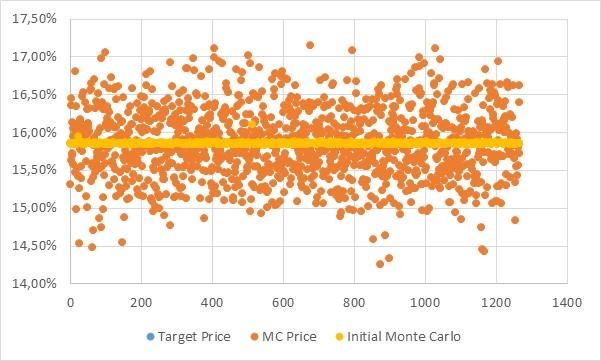
Acknowledgement & Disclaimer

Thanks to Abdelkrim Lajmi, Antoine Kremer, Luc Mathieu,
Carole Camozzi, José Luu, Rida Mahi, Claude Muller, William
Leduc, and Marouen Messaoud for useful discussions.

The opinions expressed in this presentation and on the
following slides are solely those of the presenter and not
necessarily those of Natixis.

2
Summary

1. FRTB main concepts (SA – IMA)

2. Monte Carlo optimization techniques

3   9 janvier 2017
Summary

1. FRTB main concepts (SA – IMA)

2. Monte Carlo optimization techniques

4   9 janvier 2017
A lookback at previous risk regulations

                       1996     2005    2009    2016

                       Basel    Basel   Basel   FRTB
• Basel I - 1996 : 20  pages
                       I        II      2.5

   – Regulatory capital requirements for market risk are amended to the
     overall capital requirements accord
• Basel II – 2005 : hundred of pages
   – Changes to existing market risk regime are performed in order to
     foster international convergence
• Basel 2.5 - 2009 : thousand of pages
   – Extensive amendments as consequence of the Global Financial Crisis,
     focusing on default and migration risk, and treatment of securitizations
• FRTB - 2016 : 90 pages
   – Complete overhaul of the existing framework in various areas, like risk
     measurement methods, placing a large strain on bank’s quantitative
     finance resources. Banks have to be compliant by December 31 2019

5   9 janvier 2017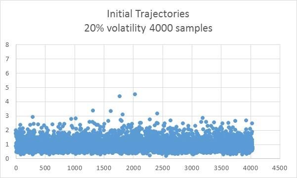
2 FRTB Main Concepts
                                      Internal Model           Banking and
        Standardized
                                         Approach             Trading Books
       Approach (SA)
                                          (IMA)                 Boundary

      • For capital               •    Switch from VaR to     •   Identification of
        requirement                    Expected Shortfall         trading accounts
        calculation                    (ES)                       and trader
      • Fallback or floor for
                                  •    Market Risk            •   Formalization of
        IMA approach
                                       Illiquidity taken          the business
      • Consideration of               into account               strategy
        hedging and
        diversification benefit   •    Default Risk Charge    •   Weekly risk
                                       (DRC)                      reporting
      • Mandatory calculation                                     requirements for
        monthly                   •    Strict regulatory          defined desks
                                       led approval
      • Generate higher
                                       process (P&L Attrib,   •   Regulatory led
        capital charges than
        IMA (TBC)                      Backtesting)               approval process
                                                                  for the proposed
      • Sensitivities based       •    Additional charge          desks
                                       for Non Modelable
      • Default risk and               Risk factors (NMRF)
        residual risk add-ons          and default risk

6   9 janvier 2017
FRTB : Eligibility to IMA
Eligibility to IMA approach per desk has to be homologated
by the regulator:

           Bank Wide     Desk Level Model
                                                   Risk Factors
           Assessment       Approval

                             Homologation

                         P&L Attribution:      At desk level:
                         • Monthly             One have to make sure
                           computation         • Real transaction
                         Test robustness         prices
                         •   Backtesting
                                               •   Sufficient
                         Fallback to SA :          observation criteria
                         • 4 breaches in 12
                           months

 7   9 janvier 2017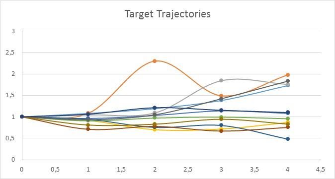
Standard Approach (SA)
                     Risk Capital Charges under Sensitivities
                                                    method
                                                                 Non Linear Risk
                                                                  (Curvature)

                                     Risk weight sensitivities

                                     Aggregate within bucket
                                                b

                                       Aggregate across
                                           buckets

8               Risk Capital Charge = Linear Risk Charge + Non
    9 janvier 2017

                Linear Risk Charge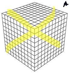
Standard Approach (SA)
Default Risk Charge challenges
Calculating the DRC consists on several computations:

• Gross JTD :
       – For each instrument, and for each equity underlying (Obligor), compute the impact of the
            default of the obligor. This step produces a gross Long / Short JTD per Obligor and per
            Instrument.

• Net JTD :
       – For each Obligor, apply a netting algorithm over all the positions of the bank to obtain a net
            Long / Short JTD per Obligor.

• Hedge Benefit :
       – Application of a partial hedge benefit ratio to account for a partial offset of long and short
            exposures in distinct Obligors.

• Risk Weights :
       – For each of the three reglementary buckets, assign a rating grade to each Obligor and
            compute the DRC per bucket using the corresponding risk weights.

9   9 janvier 2017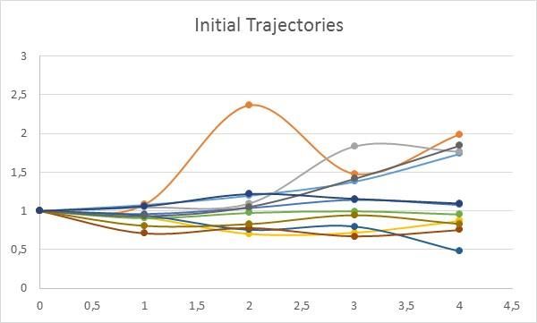
Internal Model Approach (IMA)
                                    General description

The idea is of the IMA is to better take into account :
• Tail risks
• Liquidity risk : Regulator imposed Liquidity Horizon per asset types
• Factor in default risk for select subset of asset classes
• Clearly separate modellable and non modellable risk factors
• Regulatory prescribed list of risk categories

IMA main items:
  •  A switch to from VaR to Expected Shortfall
  •  Regulator defined Liquidity horizons to be factored in ES computations
  •  Default Risk Charge
  •  Non Modellable Risk Factors

 10   9 janvier 2017
Internal Model Approach (IMA)
A switch to Expected Shortfall
• Calculated daily
• 97.5th percentile, one-tailed confidence level is to be used
• Quantitative standards
• A switch to from VaR to Expected Shortfall
• Regulator defined Liquidity horizons to be factored in ES computations
• Separate model to measure default (IMA Default Risk Charge, IMA DRC)
• Non Modellable Risk Factors
11 9 janvier 2017Internal Model Approach (IMA)
A switch to Expected Shortfall
• Stressed expected shortfall computed with all risk factors shocked
• Expected Shortfall addiotionally computed for shocks of each risk factor, all
others held constant
• T: length of the base horizon (10 days)
• ES_T(P) is ES at horizon T of a portfolio P constituted of positions p_i with respect to shocks to all risk
factors valid for positions within P
• ES_T(P, j) is the ES at horizon T (10 days) of a portfolio P (positions p_i) with respect to shocks for
each position p_i in the subset of risk factors Q(p_i, j) with all other risk factors held constant
• ES at horizon T (ES_T(P)) and ES_T(P, j) must be calculated for changes in risk factors over the time
interval T with full revaluation
• Q(p_i, j) is the subset of risk factors whose liquidity horizons for the desk where p_i is booked are at
least as long as LH_j
• The timeseries of changes in risk factors over the base time interval T (10 days) may be determined by
overlapping intervals
• LH_j Liquidity Horizon j
12 9 janvier 2017Internal Model Approach (IMA)
IMCC Calculation
Desk Level
Capital Charge
Ratio of ES on
reduced and
full RF set
Shock to RF per Liquidity Horizon
J=2 J=2
J=3 J=3
J=4 J=4
J=5 J=5
13 9 janvier 2017Summary 1. FRTB main concepts (SA – IMA) 2. Monte Carlo optimization techniques 14 9 janvier 2017
Ideas

1. Shadow grid
2. Hot Spot Monte Carlo
3. Transforming trajectories

15   9 janvier 2017
Shadow Grid
Non Parametric approach:
• We put values in a grid and proceed to the algorithm described below:
• We decompose our n dimensional cube in n 2-dimensional projections
Values in a grid with a valuation algorithm as follows:
•
We assume that we would like to calculate the function u x1 ,..., x n
0,..x ,.x , x 0 :here only two variables x ,.x have moved.
• We locate each couple of coordinates x , x within the grids.
We use a bi-cubic spline interpolation to value a bi-dimensional function vi , j u x1
i j
•
,..x ,.x 0, x 0 : here this is a special case of the previous where
i j n
i j
We use a cubic spline interpolation to value a one dimensional function
•
just one variable has moved.
ui u x1 0 i j n
• We use the reconstruction formula based on Taylor
n
u x1 ,..., x n u 0 u i u (0)
i 1
v u (0) u i u (0) u j u (0)
n n
i, j
i 1 j i 1
16 9 janvier 2017Shadow Grid
• Efficient FO pricing : Pricing grid capacity estimates
Fast Analytical prices (such as Vanillas, TRS, 7 (S) x 3 (vol) + 3(repo) + 3(div) +
Swaps) 3(rates) around 30 pricings necessary.
Slow Analytical prices (such as variance swaps
Idem.
under cash dividend assumption)
7 (S) x 3 (vol) + 3 (skew) + 3(repo) +
PDE pricing (barrier options, American options)
3(div) + 3(rates) around 33 pricings.
Monte Carlo Flow Business or Structured business
7 (S) x 3 (vol) + 3 (skew) + 3(repo) +
with a usage of aggregators (such as Volatility
3(div) + 3(rates) around 33 pricings.
swaps, Autocall on basket or worst of)
7 (S) x 3 (vol) + 3 (skew) + 3(repo) +
3(div) + 3(rates) around 33 pricings.
Based on previous analysis we have the
Monte Carlo Structured Business (general case)
possibility to use one global pricing
which randomizes the payoff and
extracts a series of grid prices.
Convertible Bonds Like a PDE approach
17 9 janvier 2017Hot Spot Data Model Diffusion • Classical simulation for pricing • Hot Spot simulation for multiple initial condition pricing 18 9 janvier 2017
Hot Spot Data Model Diffusion
• Where it comes from?

• Old recipe to stabilise the greeks within a LSM
  method

• Used in the case of the multi asset Uncertain
  volatility correlation model

19   9 janvier 2017
Hot Spot Data Model Diffusion
Efficient FO pricing
Monte Carlo Structured business (general case) : The idea is to randomize the initial conditions, combined with a
few scenario
Conceptually:
• If the pricer is f x, y where x is the state variable of the diffusion model and y is the state variables of the
data model involved in the scenario engine.
• We introduce x , the volatility of the Monte Carlo state variable and y , the volatility of the data model. We
assume that the is a correlation xy standing between the two types of variables.
Our task is to calculate the maturity scenarios.
• We extend the existing Monte Carlo by randomizing each path using the following mechanism:
x1 T , y1
x x x xy x
1 xy2 y T
Where x , y are two independent normal random variables.
20 9 janvier 2017Transforming trajectories
Efficient FO pricing through
1. Architectural building
2. Computational ordering
x
21 9 janvier 20171. DRC challenges
– Calculating the Gross Long / Short JTD per instrument and per Obligor is the first step and the
cornerstone of the DRC computation.
– It consists on simulating the default of the underlyings (Obligor per Obligor) then calculating
the impact of such defaults.
This specification raises some technical issues:
– What does it mean to simulate the default of an index (e.g. S&P 500), an ETF, a Basket, etc. ?
the FRTB guidelines specify that a look through approach should be applied.
– How should we perform the simulations such that the computation time remains bounded ?
for an exotic call option on S&P500 priced via 200K Monte Carlo simulations, should we
simulate the default of each component of the S&P 500 ? (200K*500 = 100 Millions
simulations)
– What if an Obligor exists within two underlyings of the option?
for a call option on both CAC 40 and FP Total, should we perform one global or two partial
pricings ?
22 9 janvier 20172. Look Through Approach
In order to compute the Gross JTD per Obligor for an instrument having a “non atomic” underlying
(index / ETF / Fund / Hedge Fund / Basket / etc.), we need to identify two set of parameters :
– Composition
First, we need to identify the list of Obligors on which depends each “non atomic” underlying of
the instrument.
– Shocks
Once the list of Obligors has been defined, we need to assign a shock per Obligor. In
fact, the Obligors are not directly modelled within the pricing libraries, only the “non atomic”
underlying is. Hence, we need to compute an equivalent shock : a shock of the “non atomic”
underlying that would be observed if the Obligor were to default.
23 9 janvier 20172. Look Through Approach
1) Build the tree
Non Atomic Underlying
w0 S0 w1 S1 w2 S2
w00 w22
S00 w01 S01 w02 S02 w20 S20 w21 S21 S22
FX1 FX2
S220 S221 S222 S223
w220 w222 w222 w223
FX3 FX4
2) Flatten the tree
Non Atomic Underlying
S00 S01 S02 S1 S20 S21 S220 S221 S222 S223
w00*w0*FX1 w01*w0 w02*w0 w1 W20*w2 W21*w2 W220*FX3 W222*w22 W222*w22 W223* FX4*W222
*w22*FX2*w2 *FX2*w2 *FX2*w2 *w22*FX2*w2
24 9 janvier 20172. Look Through Approach
3) Calculate the shocks
– Each shock is computed as the percentage with which the Non Atomic Underlying would vary if
Obligor i were to default (hence Si= 0)
Non Atomic Underlying
S00 S01 S02 S1 S20 S21 S220 S221 S222 S223
Shock 00 Shock 01 Shock 02 Shock 1 Shock 20 Shock 21 Shock 220 Shock 221 Shock 222 Shock 223
– Non equity underlyings are ignored (for instance, the Interest Rate Swaps within an auto-call)
except for futures on dividends where the underlying are “indirectly” impacted by the default
of the obligors
25 9 janvier 20173. Additional Pricings
– Additional Pricings are required when one Obligor belongs to the composition of two or more
underlyings of the instrument:
Non Atomic Underlying 1 Non Atomic Underlying 2
w0 S0 w1 S1
w00 w01 S w02 S02 w20
S00 S20 w21 S w22 S22
FX1
– Shocking each underlying separately to account for the Obligor default is economically not
viable : this approach is incomplete due to the uncaptured cross-sensitivity.
A separate run where both underlyings are simultaneously shocked is required !
– This functionality has been implemented in the DRC algorithm. The latter captures the need for
additional pricings, and proposes to the user to perform the computations.
– The Gross JTD may vary considerably depending on yes or no cross-sensitivities are taken into
account.
26 9 janvier 20174. Monte Carlo Optimization
– Computations are performed “within the pricing engines” and without additional
simulations. To illustrate the implemented methodology, let us consider a simple call option
on a basket of n equities (S1,…, Sn) priced via MC (100K simulations) and on which we need
to apply shocks (SH1, …, SHn) to calculate the Gross JTDs.
– The “basic” approach consists on:
looping over the shocks (SH1,…, SHn). For each shock:
-Shock the equity spot Si with the corresponding shock SHi at the data model level
-Create the pricer
-Simulate 100K trajectories
-Price the instrument
– The “Advanced” approach consists on:
building the pricer based on the baseline market context
simulating 100K trajectories
On each trajectory:
-Separately and consecutively apply the n shocks (SH1,…, SHn) then call the payoff
-Store the n intermediary calculations
Aggregate on the MC level for each shock
Basic MC Advanced MC
Pricer instances n 1
Simulations 100K*n 100K
Payoff Calls 100K*n 100K*n
27 9 janvier 20175. Pricing / Interpolation Grids
– Some non-atomic underlyings require too many repricings. Rather than performing all of them,
the DRC algorithm performs maximum 11 repricings / underlying and interpolates the others.
– To illustrate this methodology, let us consider a call option on a basket of S&P 500 and FTSE
100 priced via MC (100K simulations). Calculating the Gross JTD for this option would on
average require to apply 600 shocks.
– Rather than performing all the shocks / pricings:
we identify the maximum and minimum shocks to apply to each underlying
set up a grid of 11 shocks for this underlying
perform the pricings using these grid shocks
Interpolate the prices corresponding to the non performed shocks (interpolation time is negligible)
In our example, we apply 22 shocks (rather than 600) then perform maximum 596 interpolations
Basic MC without Advanced MC with
interpolation interpolation
Pricer instances 600 1
Simulations 600*100K 100K
Payoff 600*100K 22*100K
28 9 janvier 20176. Change of the calling architecture
– From new market data context we jump
directly to the trajectories
– We skip refining data (going from
discrete points to continuous ones)
– We skip calibration of models
– We skip generation of random numbers
– We skip the path reconstruction
– All these steps make that the overhaul
calculation is much more faster
– ……
– ??? Can we do it for non standard
scenarios ???
29 9 janvier 2017From one market data to another one
– From new market data context we jump
directly to the trajectories
– No : We skip refining data (going from
discrete points to continuous ones)
– No : We skip calibration of models
– Yes : We skip generation of random
numbers
– Yes-simpler : We skip the path
reconstruction (simple replacement)
– All these steps make that the overhaul
calculation is much more faster
– ……
– ??? Can we do it for non standard
scenarios ???
30 9 janvier 2017Approximate directly from Market data and Paths
– From new market data context we jump
directly to the trajectories
– We use this rule of thumb
and transform existing trajectories into
new ones without having to go through all
library steps.
2 different
Estimations
From From
Trajectories Market Data
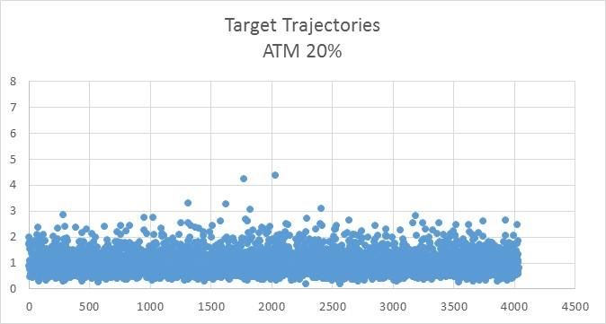
31 9 janvier 2017Example : Sanity check : go from 20% volatility 4000 samples to 20% 32 9 janvier 2017
Example : Sanity check : go from 20% volatility 4000 samples
to 20%

33   9 janvier 2017
Example : Sanity check : go from 20% volatility 4000 samples
to 20%

34   9 janvier 2017
Example : Sanity check : go from 20% volatility 4000 samples
to 20%

                      Strike                  100%   Strikes                100%
                      Analytica Price       15,85%   IV                   20,00%
                      Initial Monte Carlo   16,08%   Analytic Price       15,85%
                                                     Target Monte Carlo   15,86%

 • Normal Monte Carlo with as little as 4000
   samples does not converge to the basis point!

 • The adjustment method seems in this example
   to erase this error.

 • Can we repeat the experiment?

35   9 janvier 2017
Example : Sanity check : repeat 1500 # Monte Carlo
• This method erases
Convergence error
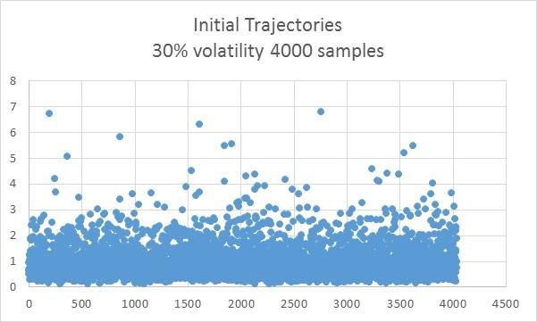
36 9 janvier 2017Example : go from 30% volatility 4000 samples to 20% + Skew 37 9 janvier 2017
Example : go from 30% volatility 4000 samples to 20% +
Skew

38   9 janvier 2017
Example : go from 30% volatility 4000 samples to 20% +
Skew

39   9 janvier 2017
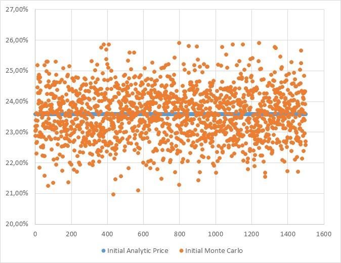
Example : go from 30% volatility 4000 samples to 20% +
Skew

       Strike                 100%    Strikes                 80%    100%     120%
       Analytica Price       23,58%   IV                   21,00%   20,00%   19,00%
       Initial Monte Carlo   24,63%   Analytic Price       26,99%   15,85%    8,42%
                                      Target Monte Carlo   27,00%   15,85%    8,42%

40   9 janvier 2017
Example : repeat 1500 # Monte Carlo
– This method erases 3 types of Errors
– Calibration
– Discretisation
– Convergence
41 9 janvier 2017Conclusion
• We have presented the computational challenge
within the FRTB framework
• We have seen detailled examples solving the
Standard method, precisely the DRC
• We have also presented several ideas to
accelerate the pricing
• Transforming the IT calling architecture
• Hot Spot simulation & trajectory
transformation
42 9 janvier 2017You can also read