Analytic Integration Methods in Quantum Field Theory
←
→
Page content transcription
If your browser does not render page correctly, please read the page content below
Analytic Integration Methods
                      in Quantum Field Theory

                          Johannes Blümlein,
                               DESY

1. Introduction
2. The Computer Algebra Landscape in Quantum Field Theory
3. Symbolic Integration of Feynman Integrals
4. Some Recent Results
5. Literature

J. Blümlein   aec 2022                        Vienna, A, July 2022   – p.1/30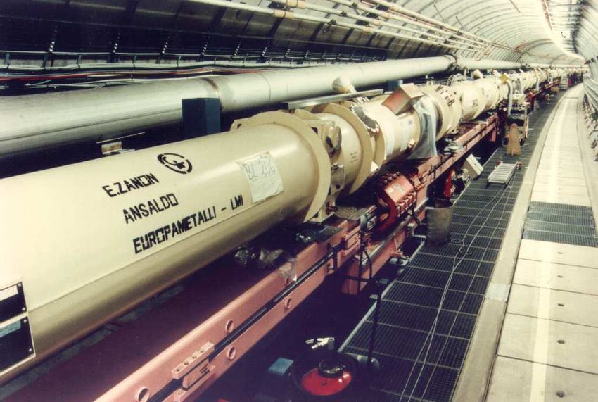
1. Introduction

Loops and Legs:
Feynman diagrams describe elementary scattering
processes between bosons and fermions in Quantum Field
Theory (QFT). Here we will thoroughly refer to
renormalizable QFTs.
Where are these techniques important?

  1. Perturbation Theory of the Standard Model and its renormalizable extensions.
  2. String amplitude calculations
  3. Perturbative calculations in Gravity
  4. non-relativistic field theories in vacuum and at finite temperature and/or density

We will calculate Feynman diagrams. These are skeletons according to Feynman rules,
connecting vertices with propagators.
They possess external lines: The Legs.
They possess internal closed lines: The Loops.
  J. Blümlein   aec 2022                         Vienna, A, July 2022                  – p.2/30

The machines, for which we perform the calculations:

                          LHC, Geneva/CH
J. Blümlein   aec 2022            Vienna, A, July 2022      – p.3/30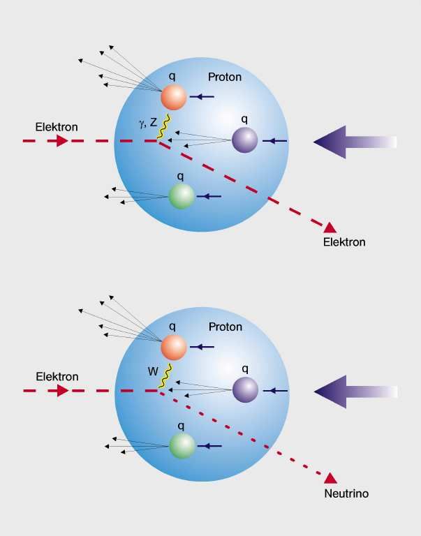
HERA, Hamburg/D          microscopy of the proton

J. Blümlein   aec 2022   Vienna, A, July 2022       – p.4/30

Why are these calculations important ?

1. Precision extraction of coupling constants: αs (MZ )@1%
2. Do couplings unite at high scales and in which field
   theories?
3. Precision measurements of mc , mb , mt at LHC and a
   future ILC
4. Precision understanding of the Higgs and top sector (at
   the LHC, ILC and possibly other machines)
5. Unravel the mathematical structure of microscopic
   processes analytically: get further with the
   Stueckelberg-Feynman programme as far as you can.
   =⇒      Genetic Code of the Micro Cosmos
 J. Blümlein   aec 2022        Vienna, A, July 2022         – p.5/30
2. The Computer Algebra Landscape in Quantum Field Theory

 The pioneers:

                 M. Veltman                                               A.C. Hearn
                 Schoonschip                                                Reduce
                                   both started 1963
                      (1999)

  1. Almost all calculations in QFT were performed using these packages          < 1989.
                                                                                 ∼

  2. The renormalizibility proof of the SM needed Schoonschip to be verified in its details.
  3. Level: 1- and 2-loop calculations mostly; first 3-loop calculations.

  J. Blümlein   aec 2022                          Vienna, A, July 2022                       – p.6/30
The Computer Algebra Landscape in Quantum Field Theory Many symbolic systems and packages written using various languages are in use and will be in use in the future. 1. Fortran, C 2. Mathematica 3. Maple 4. FORM 5. GiNac 6. Sage 7. Pari, and others • Many calculations bind different packages by shell-scripts to a general computer-algebraic work-flow to solve large-scale problems. • Condition: the average time used in the parts is not tiny. • Allows for natural checkpoints; in- and output pattern has to be provided in an automated form. Our computer-algebra cluster currently consists of more than 10 units with ∼ 16 Tbyte RAM and ∼ 230 Tbyte fast disc together; we use hundreds of Mathematica licenses. J. Blümlein aec 2022 Vienna, A, July 2022 – p.7/30
The main steps of a typical large scale calculation

1. Generate the Feynman diagrams: O(100 − 100.000) package QGRAF [Fortran]
   P. Nogueira
2. Calculate all group theoretic structures: package COLOR [FORM]
   T. van Ritbergen et al.
3. Perform all tensor and Dirac-matrix calculations in 4 + ε dimensions, perform all radial
   momentum integrals: package FORM; J. Vermaseren
   remaining: Feynman parameter integrals.

                             1. FORM (since the late 80ies) became the
                                most powerful C-programme to perform particle
                                physics calculations. It is a specialized package.
                             2. Efficient treatment of giant number of terms,
                                very good memory management, several paral-
                                lelization possibilities
                             3. Several additional packages: e.g. special num-
                                bers, harmonic sums, harmonic polylogarithms
                             4. Implementation of 4-loop master integrals, R∗
 J. Vermaseren
                                renormalization operation; allows for several 5-
                                loop calculations.
J. Blümlein   aec 2022                          Vienna, A, July 2022                         – p.8/30
The main steps of a typical large scale calculation
4. Alternatively: reduce to a small number of scalar master integrals, to be calculated by
other methods.
5. All accessible Gauß-Stokes integrals are used to reduce millions of scalar integrals
often to O(100 − 5000) master integrals; different codes. Examples: S. Laporta,
Anastasiou, Studerus/Manteuffel: Reduze2, Marquard, Lee, and many more.
Example: 3-loop heavy flavor corrections to DIS
[S. Wolfram computed the 1-loop correction in 1978, after E. Witten 1976]
The reduction to master integrals produces 1.6 Tbyte C-output of relations to determine the
master integrals.
100.000ds of scalar integrals =⇒ 687 3-loop master integrals.
In the calculation of the master integrals Mathematica plays
a key-role.
J. Blümlein aec 2022 Vienna, A, July 2022 – p.9/30Cooperation with the Research Institute of Symbolic Computation
1. Symbolic summation and integration in
difference field theory
2. Symbolic solution of large differential
equation systems
3. Special functions and numbers in QFT
4. Modular forms and functions, q-series
C. Schneider J. Ablinger P. Paule, chairman of RISC
Mathematica packages :
1. Sigma (C.S.)
2. EvaluateMultSums, Sumproduction, SolveCoupledSystems (C.S)
3. HarmonicSums, MultiIntegrate (J.A.)
4. RhoSum (M. Round)
J. Blümlein aec 2022 Vienna, A, July 2022 – p.10/303. Symbolic Integration of Feynman Integrals
1. Integration by parts technique
2. Mellin-Barnes techniques
3. PSLQ: zero-dimensional integrals
4. Guessing: one-dimensional integrals [M. Kauers]
5. Generalized hypergeometric functions (and extensions)
6. Risch algorithms [C.G. Raab]
7. Solution of master-integrals using difference and differential
equations
8. Summation techniques: construction of difference rings and
fields
9. (multivalued) Almkvist-Zeilberger algorithm ... and others.
10. The method of arbitrary high moments
J. Blümlein aec 2022 Vienna, A, July 2022 – p.11/30Function Spaces
Sums Integrals Special Numbers
Harmonic Sums Harmonic Polylogarithms multiple zeta values
N k Z x Z 1
1 X (−1)l dy y dz Li3 (x)
X Z
dx = −2Li4 (1/2) + ...
k=1
k l=1
l3 0 y 0 1+z 0 1+x
gen. Harmonic Sums gen. Harmonic Polylogarithms gen. multiple zeta values
N k Z 1
(1/2)k X (−1)l
Z x
dy y dz ln(x + 2)
X Z
dx = Li2 (1/3) + ...
k=1
k l=1
l3 0 y 0 z−3 0 x − 3/2
Cycl. Harmonic Sums Cycl. Harmonic Polylogarithms cycl. multiple zeta values
N k Z x Z y ∞
X 1 X (−1)l dy dz X (−1)k
C=
k=1
(2k + 1) l=1 l3 0 1+y
2
0 1−z+z
2
k=0
(2k + 1)2
Binomial Sums root-valued iterated integrals associated numbers
N Z x
1 2k dy y dz √
X Z
(−1) k
√ H8,w3 = 2arccot( 7)2
k=1
k2 k 0 y 0 z 1+z
non-iterating integrals. associated numbers
z 4 5 2 (x2 − 9)2 Z 1 4 5 2 (x2 − 9)2
ln(x) , x , x
Z
dx 3 3 ; dx 2 F1 3 3 ;
2 F1
0 1+x 2 (x2 + 3)3 0 2 (x2 + 3)3
shuffle, stuffle, and various structural relations =⇒ algebras
J. Blümlein aec 2022 Vienna, A, July 2022 – p.12/30integral representation (inv. Mellin transform)
Function Spaces
S-Sums H-Sums C-Sums C-Logs H-Logs G-Logs
S1,2 1 , 1; n S−1,2 (n) S(2,1,−1) (n) H(4,1),(0,0)(x) H−1,1 (x) H2,3 (x)
2
x →c∈R
Mellin transform
n→∞
x →1
x →1
S1,2 1 , 1; ∞ S−1,2 (∞) S(2,1,−1) (∞) H(4,1),(0,0)(1) H−1,1 (1) H2,3 (c)
2
power series expansion
2i
square-root valued letters ⇐⇒ nested binomial sums i
non-iterative iterative integrals =⇒ Iterate on non-it. integrals with rat. 1 / 1
argument (complete elliptic integrals) [arXiv:1706.01299]
J. Blümlein aec 2022 Vienna, A, July 2022 – p.13/30The PSLQ-Method
Seek an Integer Relation over a basis of special numbers
out of a special class.
Example: Z 1
Li3 (x)
I= dx
0 1+x
The integral is of “transcendentality” τ = 4.
The expected HPL(1) basis is spanned by:
ln4 (2), ln(2)ζ3 , ln2 (2)ζ2 , ζ22 , Li4 (1/2).
Calculate this integral numerically to high number of digits, e.g. 40 digits.
I ≈ 0.3395454690873598695906678484608602061388
The PSLQ algorithm yields:
π4
1 4 3 1 2 1
I = − ln (2) + + ln(2)ζ3 + ln (2)π 2 −2Li4
12 60 4 12 2
2k B
k−1 (2π) 2k
ζ2k = (−1) ; Bn [Bernoulli number]
2(2k)!
J. Blümlein aec 2022 Vienna, A, July 2022 – p.14/30Guessing Difference Equations
It is often easier to calculate Mellin moments for a quantity
for fixed values of N than to derive the relation for general
values of N in the first place. If the quantity under
consideration is known to be recurrent than its difference
equation is of finite order and degree.
O
(l)
X
∃ Pk (N )F (k + N ) = 0; max{l} - degree; O - order
k=0
Example:
−(N + 1)3 F (N ) − (3N 2 − 9N − 7)F (N + 1) + (N + 2)3 F (N + 2) = 0
1
F (1) = 1; F (2) =
8
N
X 1
Solution: F (N ) = 3
= S3 (N )
k=1
k
J. Blümlein aec 2022 Vienna, A, July 2022 – p.15/30Guessing Difference Equations Solution of large problems Assume you would like to calculate the massless 3-loop Wilson coefficients in deep-inelastic scattering using this method. How many moments would you need and how do they look like ? About 5200 moments are needed. The largest ones are ratios of #13000/#13000 digits. They can be calculated within 15 min. After 3 weeks you weree needed in 2009 find a difference equation of degree ∼ 1000 and order 35, if you have a reasonable computer (100 Gbyte RAM). After another week you have the solution as function of N . [Now all times are much smaller: a few days only.] Problem: It is sophisticated to obtain the input a priori. Combined solution-methods do work, however, to O(1500) moments. Recent results: 3-loop anomalous dimension computed from scratch. [arXiv:1701.04614, 1705.01508, 1908.03779, 2107.06267, 2111.12401]. J. Blümlein aec 2022 Vienna, A, July 2022 – p.16/30
Generalized Hypergeometric Functions

At lower number of legs and/or loops Feynman integrals happen to
be represented by these functions.
After suitable mappings these functions have compact
representations in infinite (multiple) absolutely convergent sums.
This allows for the Laurent-expansion in ε under the summation
operator.
Important Examples:
  1. B(a, b)
  2.    p Fq (ai ; bj ; x);   always single sums
  3. Appell functions; double sums
  4. Kampé de Feriet functions, Horn functions and higher; more sums [cf. 2111.15501]

The sums may be expanded and summed using algorithms like
nestedsums, xsummer, HarmonicSums, Sigma, EvaluateMultiSums

 J. Blümlein   aec 2022                           Vienna, A, July 2022                 – p.17/30
Generalized Hypergeometric Functions

Example:
Integrals of the following type emerge:
                                 Z     1                       Z       1
                                              δ            η
                I1 (z)     =               dyy (1 − y)                     dxxβ−1 (1 − x)γ−β−1 (1 − xyz)−α
                                   0                               0
                                                   Z       1
                           =     B(β, γ − β)                   dyy δ (1 − y)η          2 F1 (α, β; γ; yz)
                                                       0
                           =     B(β, γ − β)B(δ, η − δ)                      3 F2 (δ, α, β; η, γ; z)

All p Fq ’s have single series representations. One series counts as one integral.

                                                                 ∞
                                                                X   (a1 )k ...(ap )k z k
                           p Fq (a1 , ..., ap ; b1 ...bq ; z) =
                                                                k=0
                                                                    (b1 )k ...(bq )k k!

 J. Blümlein   aec 2022                                                       Vienna, A, July 2022          – p.18/30
Summation Techniques
The integrals can usually be traded for a lower number of sums
(finite or infinite).
Solve these sums for N and/or in terms of special constants.
Principal Idea:
1. Sums may be represented in vector spaces, algebras, and finally fields/rings
2. Rephrase the sums in the setting of difference fields and rings
3. Apply telescoping, creative telescoping, and other principles in this setting to compute
recurrences
4. Try to solve the recurrences; possible for most sums occurring from Feynman integrals
5. In addition, use nested sums algebras to speed up calculations
Telescoping: Find a function g(k) such
f (k) = g(k + 1) − g(k)
N
X
F (N ) = f (k) = g(N + 1) − g(1)
k=1
=⇒ nested sums algebras =⇒ bases
Sigma solves large scale problems running over months and using
several hundred Gb RAM.
J. Blümlein aec 2022 Vienna, A, July 2022 – p.19/30Differential Equations The IBPs deliver a vast amount of differential equations forming systems, which are nested hierarchically. Provide boundary conditions [usually using other methods] Perform uncoupling of these systems • In case of complete 1st order uncoupling: ∃ complete solution algorithm in case of any basis choice for 1 parameter systems All solutions are iterative integrals over whatsoever alphabet: x R 0 dyfa (y)H~b (y) • Irreducible nth order systems (n ≥ 2): present target of research even in mathematics; good prospects in case of 2nd order systems [convergent near integer power series (CIS)] At least one function is given by a definite integral, others iterate on. =⇒ iterated integral algebras =⇒ bases J. Blümlein aec 2022 Vienna, A, July 2022 – p.20/30
The Almkvist-Zeilberger Algorithm

• Given a multiple integral over hyperexponential terms:
         R1             Ql
F (n) = 0 dx1 ...dxj k=1 (P (xi , n))rk ,ǫ , rk ∈ R and n ∈ N a
parameter.
                         Pm
• Find a recurrence: k=0 pk (n, ǫ)F (n + k) = H(n, ǫ) with some
inhomogeneity H(n, ǫ).
• Correspondingly n → x, a differential equation:
Pm                dk
   k=0 pk (x, ǫ) dxk F (x) = K(x, ǫ) with some inhomogeneity K(x, ǫ).
Either the inhomogeneities can be forced to vanish, or a hierarchy
of equations has to be solved using summation techniques and
DEQ-solvers (which may also be summation techniques).

 J. Blümlein   aec 2022              Vienna, A, July 2022              – p.21/30
The method of arbitrary high moments • 0–scale problems are simpler to solve than 1–scale problems • Mellin moments can be obtained for fixed values of N ∈ N and satisfy the difference equations, obtained from the differential equations due to the IBP relations for the master integrals. • One generates large enough sets of moments for master integrals (at the moment up to 10000.) • The master integrals are inserted into the final amplitude. Here lots of potential non-first order factorizing terms cancel. • Guessing is used to obtain corresponding recurrences. • In quite a series of cases these recurrences factorize to first order and Sigma can solve these recurrences. • Otherwise non-first order factorizing terms can all be split off. Other technologies are needed to proceed, which are currently developed. [1701.04614] J. Blümlein aec 2022 Vienna, A, July 2022 – p.22/30
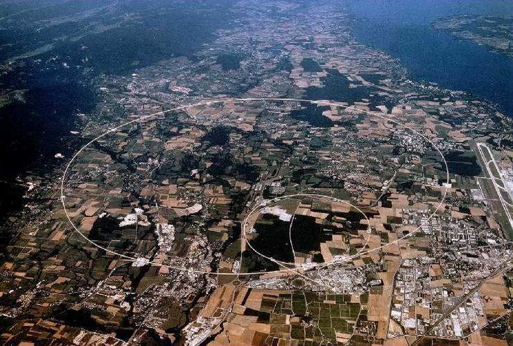
The present NC corrections to F2 (x, Q2 )
                                                                             αs      αs2   αs3
                         0.06                                 HgS,2 /20
                                                                     PS
                                                                  Hq,2
                         0.04                                      LNS
                                                                     q,2
                                                                     S
                                                                   Lg ,2
                         0.02                                      LPS
                                                                     q,2

                            0
               F2heavy

                         -0.02
                                                  0.001

                         -0.04                            0

                         -0.06                    -0.001

                         -0.08                    -0.002
                                                                  10−1                      1
                             10−5   10−4   10−3           10−2                10−1               1
                                                  x

               Q2 = 100 GeV2 , Hg,2
                                S scaled down by a factor 20.

J. Blümlein       aec 2022                           Vienna, A, July 2022                           – p.23/30
The Strength of Mathematica and Possible Improvements All our symbolic integration codes are written in Mathematica. • Over the years they were steadily improved and extended. • Mathematica’s rich special function implementations and the strong integrator are most helpful. • This also applies to the math world’s pages and detailed on-line tabulations of other kind. • Freeing memory in Mathematica which is no longer used would be instrumental in some cases. We operate jobs with a RAM request of up to ∼ 500 Gbyte and sometimes face difficulties. • Dynamic outsourcing to fast disc, like available in FORM, would be very helpful. • In some cases relying heavily on very fast integer arithmetics we had to use Sage because of the size and run time requests of our current problems. J. Blümlein aec 2022 Vienna, A, July 2022 – p.24/30
4. What can be achieved by all that ?

• A lot of integration technology has been created for many analytic
  precision calculations for the Large Hadron Collider and the
  planned International Linear Collider.
• The results allow also for many advanced solutions in
  combinatorics and number theory.
• Within elementary particle physics the present results allow to
  improve the precision of two fundamental constants of the
  Standard Model:

                           δαs (MZ )
                                     < 1%    δmc < 20MeV
                           αs (MZ )

which may have consequences for various proposed extensions
of the SM.
 J. Blümlein   aec 2022                    Vienna, A, July 2022       – p.25/30
4. What can be achieved by all that ? • Detailed exploration of the tt̄ sector for new physics • QCD background predictions in the search of unexpected signals by new particles • At the theory side: 4–loop calculations of the scaling violations of parton distribution functions in the future • Also: crucial tests for small x predictions. • Computer algebra calculations in the 10-100 Gbyte region, lasting various CPU years. • Still analytic solutions are possible. J. Blümlein aec 2022 Vienna, A, July 2022 – p.26/30
5. Literature
  References

   1. A recent review: J. Ablinger and J. Blümlein, arXiv:1304.7071 [math-ph].
   2. Graph Polynomials: N. Nakanishi, Suppl. Progr. Theor. Phys. 18 (1961) 1–125; Graph
      Theory and Feynman Integrals, (Gordon and Breach, New York, 1970);                               References
      C. Bogner and S. Weinzierl, Int. J. Mod. Phys. A 25 (2010) 2585–2618 [arXiv:1002.3458
      [hep-ph]];                                                                                        1. Iterated Integrals: H. Poincaré, Acta Math. 4 (1884) 201–312;
      S. Weinzierl, arXiv:1301.6918 [hep-ph].                                                              J.A. Lappo-Danilevsky, Mémoirs sur la Théorie des Systèmes Différentielles Linéaires,
   3. Harmonic Sums: J. A. M. Vermaseren, Int. J. Mod. Phys. A 14 (1999) 2037–2076 [hep-                   (Chelsea Publ. Co, New York, NY, 1953);
      ph/9806280];                                                                                         K.T. Chen, Trans. A.M.S. 156 (3) (1971) 359–379;
      J. Blümlein and S. Kurth, Phys. Rev. D 60 (1999) 014018 [hep-ph/9810241].                            A. Jonquière, Bihang till Kongl. Svenska Vetenskaps-Akademiens Handlingar 15 (1889) 1–
   4. Shuffle- Algebraic Relations: M.E. Hoffman,                J. Algebraic Combin., 11 (2000)
                                                                                                           50;
      49–68, [arXiv:math/9907173 [math.QA]]; Nucl. Phys. (Proc. Suppl.) 135 (2004) 215
                                                                                                           E. Remiddi, J. A. M. Vermaseren and , Int. J. Mod. Phys. A 15 (2000) 725–754 [hep-
      [arXiv:math/0406589];
                                                                                                           ph/9905237];
      J. Blümlein, Comput. Phys. Commun. 159 (2004) 19–54, [hep-ph/0311046];
                                                                                                           T. Gehrmann and E. Remiddi, Comput. Phys. Commun. 141 (2001) 296–312 [arXiv:hep-
      J. M. Borwein, D. M. Bradley, D. J. Broadhurst and P. Lisonek, Trans. Am. Math. Soc. 353
                                                                                                           ph/0107173];
      (2001) 907–941, [math/9910045 [math-ca]].
                                                                                                           J. Vollinga and S. Weinzierl, Comput. Phys. Commun. 167 (2005) 177–194 [arXiv:hep-
   5. Hopf Algebras: H. Hopf, Ann. of Math. 42 (1941) 22–52;
                                                                                                           ph/0410259].
      J. Milner and J. Moore, Ann. of Math. 81 (1965) 211–264;
                                                                                                        2. Generalized Harmonic Sums: A. B. Goncharov. Mathematical Research Letters, 5 (1998)
      M.E. Sweedler, Hopf Algebras, (Benjamin, New York, 1969).
   6. Structural Relastions of Harmonic Sums: J. Blümlein, Comput. Phys. Commun. 180                       497–516, [arXiv:1105.2076 [math.AG]];
      (2009) 2218–2249, [arXiv:0901.3106 [hep-ph]];                                                        S.-O. Moch, P. Uwer and S. Weinzierl, J. Math. Phys. 43 (2002) 3363–3386, [hep-
      J. Ablinger, J. Blümlein and C. Schneider, DESY 13–064.                                              ph/0110083];
   7. Sum-Function Bases in QFT: J. Blümlein and V. Ravindran, Nucl. Phys. B 716 (2005) 128–               J. Ablinger, J. Blümlein and C. Schneider, arXiv:1302.0378 [math-ph].
      172 [hep-ph/0501178], Nucl. Phys. B 749 (2006) 1–24 [hep-ph/0604019];                             3. Cyclotomic Harmonic Sums, Polylogarithms, and Constants: J. Ablinger, J. Blümlein and
      J. Blümlein and S. Klein, PoS ACAT (2007) 084 [arXiv:0706.2426 [hep-ph]].                            C. Schneider, J. Math. Phys. 52 (2011) 102301, [arXiv:1105.6063 [math-ph]].
   8. Lyndon Words and Basis Counting: R.C. Lyndon, Trans. Amer. Math. Soc. 77 (1954) 202–              4. Binomial-weighted Nested Generalized Harmonic Sums: J. Ablinger, J. Blümlein, C.
      215; 78 (1955) 329–332;                                                                              Raab, C. Schneider, and F. Wißbrock, DESY 13–063.
      C. Reutenauer, Free Lie algebras. (Oxford, University Press, 1993);                               5. Periods: M. Kontsevich and D. Zagier, IMHS/M/01/22, in B. Engquist and W. Schmid, Eds.,
      D.E. Radford, J. Algebra, 58 (1979) 432–454;                                                         Mathematics unlimited - 2001 and beyond, (Springer, Berlin, 2011), pp. 771–808;
      E. Witt, Journ. Reine und Angew. Mathematik, 177 (1937) 152–160; Math. Zeitschr. 64                  C. Bogner and S. Weinzierl, J. Math. Phys. 50 (2009) 042302 [arXiv:0711.4863 [hep-th]].
      (1956) 195–216.                                                                                   6. Zeta Values: D. Zagier, in : First European Congress of Mathematics, Vol. II, (Paris, 1992),
   9. Factorial Series: N. Nielsen, Handbuch der Theorie der Gammafunktion, (Teubner, Leipzig,             Progr. Math., 120, (Birkhäuser, Basel–Boston, 1994), 497–512; J. Blümlein, D. J. Broadhurst
      1906); reprinted by (Chelsea Publishing Company, Bronx, New York, 1965);                             and J. A. M. Vermaseren, Comput. Phys. Commun. 181 (2010) 582–625, [arXiv:0907.2557
      E. Landau, Über die Grundlagen der Theorie der Fakultätenreihen, S.-Ber. math.-naturw. Kl.           [math-ph]] and references therein;
      Bayerische Akad. Wiss. München, 36 (1906) 151–218.                                                   J.Kuipers and J.A.M.Vermaseren arXiv:1105.1884 [math-ph];
  10. Analytic Continuation of Harmonic Sums: J. Blümlein, Comput. Phys. Commun. 133                       M.E. Hoffman’s page http://www.usna.edu/Users/math/∼meh/biblio.html;
      (2000) 76–104, [hep-ph/0003100];                                                                     S. Fischler, Sém. Bourbaki, Novembre 2002, exp. no. 910, Asterisque 294 (2004) 27–62,
      J. Blümlein and S.-O. Moch, Phys. Lett. B 614 (2005) 53–61, [hep-ph/0503188];                        http://www.math.u-psud.fr /∼fischler/publi.html;
      see also the References und Structural Relations.                                                    P. Colmez, in: Journées X-UPS 2002. La fontion zêta. Editions de l’Ecole polytechnique,
      A. V. Kotikov and V. N. Velizhanin, hep-ph/0501274.                                                  Paris, 2002, 37–164, http://www.math.polytechnique.fr/xups/vol02.html;
  11. Di- and Polylogarithms: L. Lewin, Dilogarithms and associated functions, (Macdonald,                 M. Waldschmidt, Number Theory and Discrete Mathematics, Editors: A.K. Agarwal, B.C.
      London, 1958);                                                                                       Berndt, C.F. Krattenthaler, G.L. Mullen, K. Ramachandra and M. Waldschmidt, (Hindustan
      A. N. Kirillov, Prog. Theor. Phys. Suppl. 118 (1995) 61–142, [hep-th/9408113];                       Book Agency, 2002), 1–12;
      L.C. Maximon, Proc. R. Soc. A459 (2003) 2807–2819;                                                   M. Waldschmidt, Journal de théorie des nombres de Bordeaux, 12 (2) (2000) 581–595;
      D. Zagier, Journal of Mathematical and Physical Sciences 22 (1988) 131–145; in P. Cartier,           M. Huttner and M. Petitot, Arithmeétique des fonctions d’zetas et Associateur de Drinfel’d,
      B. Julia, B.; P. Moussa et al.,Eds., Frontiers in Number Theory, Physics, and Geometry II - On       (UFR de Mathématiques, Lille, 2005);
      Conformal Field Theories, Discrete Groups and Renormalization, (Springer, Berlin, 2007) 3–           C. Hertling, AG Mannheim-Heidelberg, SS2007;
      65;                                                                                                  P. Cartier, Sém. Bourbaki, Mars 2001, 53e année, exp. no. 885, Asterisque 282 (2002)
      L. Lewin, Polylogarithms and associated functions, (North Holland, New York, 1981);                  137–173.
      A. Devoto and D. W. Duke Riv. Nuovo Cim. 7N6 (1984) 1–39;
      N. Nielsen, Nova Acta Leopold. XC Nr. 3 (1909) 125–211;
      K. S. Kölbig, J. A. Mignoco, E. Remiddi and , BIT 10 (1970) 38–74;
      K. S. Kölbig, SIAM J. Math. Anal. 17 (1986) 1232–1258.

J. Blümlein         aec 2022                                                                          Vienna, A, July 2022                                                                               – p.27/30
5. Literature
References
References
1. Number of Zeta Values: A.B. Goncharov, Multiple polylogarithms and mixed Tate motives,
arxiv:math.AG/0103059; 22. Hyperlogarithms: F. Brown, Commun. Math. Phys. 287 (2009) 925 [arXiv:0804.1660
T. Terasoma, Mixed Tate Motives and Multiple Zeta Values, Invent. Math. 149 (2) (2002) [math.AG]];
339–369, arxiv:math.AG/010423; J. Ablinger, J. Blümlein, A. Hasselhuhn, S. Klein, C. Schneider and F. Wißbrock, Nucl.
P. Deligne and A.B. Goncharov, Groupes fondamentaux motiviques de Tate mixtes, Ann. Sci. Phys. B 864 (2012) 52 [arXiv:1206.2252 [hep-ph]];
Ecole Norm. Sup., Série IV 38 (1) (2005) 1–56; E. Panzer, Comput. Phys. Commun. 188 (2015) 148 [arXiv:1403.3385 [hep-th]].
D. J. Broadhurst, arXiv:hep-th/9604128; 23. Risch algorithms: M. Bronstein, Symbolic Integration I: Transcendental Functions,
D. J. Broadhurst and D. Kreimer, Phys. Lett. B 393 (1997) 403–412 [arXiv:hep-th/9609128];
(Springer, Berlin, 1997);
F. Brown, Annals of Math. 175 (1) (2012) 949–976;
V.V. Zudilin, Uspekhi Mat. Nauk 58 (1) 3–22. C. Raab, Definite Integration in Differential Fields, PhD Tesis, August 2012, Johannes
2. Hypergeometric Functions and Generalizations: P. Appell, Sur Les Fonctions Kepler University Linz.
Hypérgéometriques de Plusieurs Variables, (Gauthier-Villars, Paris, 1925); 24. Hopf Algebras and Renormalization: A. Connes and D. Kreimer, Commun. Math.
P. Appell and J. Kampé de Fériet, Fonctions Hypérgéometriques; Polynômes d’Hermite, Phys. 210 (2000) 249 [hep-th/9912092]; Commun. Math. Phys. 216 (2001) 215 [hep-
(Gauthier-Villars, Paris, 1926); th/0003188].
W.N. Bailey, Generalized Hypergeometric Series, (Cambridge University Press, Cambridge, 25. Integration by parts techniques. J. Lagrange, Nouvelles recherches sur la nature
1935); et la propagation du son, Miscellanea Taurinensis, t. II, 1760-61; Oeuvres t. I, p. 263;
A. Erdélyi (ed.), Higher Transcendental Functions, Bateman Manuscript Project, Vol. I, C.F. Gauß, Theoria attractionis corporum sphaeroidicorum ellipticorum homogeneorum
(McGraw-Hill, New York, 1953); methodo novo tractate, Commentationes societas scientiarum Gottingensis recentiores,
H. Exton, Multiple Hypergeometric Functions and Applications, (Ellis Horwood Limited,
Vol III, 1813, Werke Bd. V pp. 5-7;
Chichester, 1976); Integrals, (Ellis Horwood Limited, Chichester, 1978);
L.J. Slater, Generalized Hypergeometric Functions, (Cambridge University Press, Cam- G. Green, Essay on the Mathematical Theory of Electricity and Magnetism,
bridge, 1966). Nottingham, 1828 [Green Papers, pp. 1-115];
3. Mellin-Barnes Integrals: E.W. Barnes, Proc. Lond. Math. Soc. (2) 6 (1908) 141; Quart. M. Ostrogradski, Mem. Ac. Sci. St. Peters., 6, (1831) 39;
Journ. Math. 41 (1910) 136–140; K. G. Chetyrkin, A. L. Kataev and F. V. Tkachov, Nucl. Phys. B 174 (1980) 345;
H. Mellin, Math. Ann. 68 (1910) 305–337; S. Laporta, Int. J. Mod. Phys. A 15 (2000) 5087 [hep-ph/0102033];
J. Gluza, K. Kajda and T. Riemann, Comput. Phys. Commun. 177 (2007) 879–893 C. Studerus, Comput. Phys. Commun. 181 (2010) 1293 [arXiv:0912.2546
[arXiv:0704.2423 [hep-ph]]. [physics.comp-ph]];
4. Summation in Difference and Productfields: C. Schneider, Discrete Math. Theor. Comput. A. von Manteuffel and C. Studerus, arXiv:1201.4330 [hep-ph].
Sci. 6 (2004) 365–386; J. Differ. Equations Appl., 11(9) (2005) 799–821; Advances in Ap- 26. Use of Differential Equations: A. V. Kotikov, Phys. Lett. B 254 (1991) 158;
plied Math., 34(4) (2005) (4) 740–767; Annals of Combinatorics, 9(1) (2005) 75–99; Sem.
E. Remiddi, Nuovo Cim. A 110 (1997) 1435 [hep-th/9711188];
Lothar. Combin., 56 (2007) 1–36; J. Symb. Comp., 43(9) (2008) 611–644 arXiv:0808.2543
[cs.SC]; Ann. Comb., 14(4) (2010) 533–552 arXiv:0808.2596 [cs.SC]; Appl. Algebra Engrg. M. Caffo, H. Czyz, S. Laporta and E. Remiddi, Acta Phys. Polon. B 29 (1998) 2627
Comm. Comput., 21(1) (2010) 1–32; In A. Carey, D. Ellwood, S. Paycha, and S. Rosenberg, [hep-th/9807119]; Nuovo Cim. A 111 (1998) 365 [hep-th/9805118];
editors, Motives, Quantum Field Theory, and Pseudodifferential Operators, 12 of Clay Math- T. Gehrmann and E. Remiddi, Nucl. Phys. B 580 (2000) 485 [hep-ph/9912329];
ematics Proceedings, pages 285–308. Amer. Math. Soc., (2010), arXiv:0904.2323 [cs.SC]. J. Ablinger, A. Behring, J. Blümlein, A. De Freitas, A. von Manteuffel and C. Schneider,
5. Hyperlogarithms: F. Brown, Commun. Math. Phys. 287 (2009) 925 [arXiv:0804.1660 Comput. Phys. Commun. 202 (2016) 33 [arXiv:1509.08324 [hep-ph]];
[math.AG]]; J.M. Henn, Phys. Rev. Lett. 110 (2013) 251601 [arXiv:1304.1806 [hep-th]].
J. Ablinger, J. Blumlein, A. Hasselhuhn, S. Klein, C. Schneider and F. Wißbrock, Nucl. Phys. 27. Irreducible Systems of Order larger than one, Elliptic Integrals : S. Laporta and
B 864 (2012) 52 [arXiv:1206.2252 [hep-ph]]. E. Remiddi, Nucl. Phys. B 704 (2005) 349 [hep-ph/0406160];
6. Risch algorithms: M. Bronstein, Symbolic Integration I: Transcendental Functions, L. Adams, C. Bogner and S. Weinzierl, J. Math. Phys. 54 (2013) 052303
(Springer, Berlin, 1997);
[arXiv:1302.7004 [hep-ph]];
C. Raab, Definite Integration in Differential Fields, PhD Tesis, August 2012, Johannes Kepler
University Linz. L. Adams, C. Bogner and S. Weinzierl, J. Math. Phys. 56 (2015) no.7, 072303
7. Hopf Algebras and Renormalization: A. Connes and D. Kreimer, Commun. Math. Phys. [arXiv:1504.03255 [hep-ph]].
210 (2000) 249 [hep-th/9912092]; Commun. Math. Phys. 216 (2001) 215 [hep-th/0003188].
J. Blümlein aec 2022 Vienna, A, July 2022 – p.28/305. Literature
More recent results:
J. Ablinger, J. Blümlein, A. De Freitas, M. van Hoeij, E. Imamoglu, et al. J. Math. Phys.
59 (2018) no.6, 062305 [arXiv:1706.01299 [hep-th]];
J. Brödel, C. Duhr, F. Dulat and L. Tancredi, JHEP 05 (2018) 093 [arXiv:1712.07089
[hep-th]]; J. Brödel, C. Duhr, F. Dulat, B. Penante and L. Tancredi, JHEP 08 (2018) 014
[arXiv:1803.10256 [hep-th]].
J. Blümlein and C. Schneider, Analytic computing methods for precision calculations in quantum
field theory, Int. J. Mod. Phys. A 33 (2018) no.17, 1830015 [arXiv:1809.02889 [hep-ph]].
J. Ablinger, J. Blümlein, M. Round and C. Schneider, Comput. Phys. Commun. 240
(2019) 189-201 [arXiv:1809.07084 [hep-ph]].
J. Ablinger, J. Blümlein, P. Marquard, N. Rana and C. Schneider, Nucl. Phys. B 939
(2019) 253-291 [arXiv:1810.12261 [hep-ph]].
J. Ablinger, J. Blümlein and C. Schneider, Phys. Rev. D 103 (2021) no.9, 096025
[arXiv:2103.08330 [hep-th]].
J. Blümlein, M. Saragnese and C. Schneider, Hypergeometric Structures in Feynman Integrals
[arXiv:2111.15501 [math-ph]].
J. Blümlein aec 2022 Vienna, A, July 2022 – p.29/305. Literature
Recent Survey Volumes:
Computer Algebra in Quantum Field Theory: Integration, Summation and
Special Functions eds.: C. Schneider and J. Blümlein, Texts & Monographs in
Symbolic Computation, (Springer, Wien, 2013).
Elliptic Integrals, Elliptic Functions and Modular Forms in Quantum Fueld Theory
eds.: J. Blümlein, C. Schneider and P. Paule, Texts & Monographs in Symbolic
Computation, (Springer, Heidelberg, 2019).
Anti-Differentiation and the Calculation of Feynman Amplitudes, eds.:
J. Blümlein and C. Schneider, Texts & Monographs in Symbolic Computation,
(Springer, Heidelberg, 2021).
J. Blümlein aec 2022 Vienna, A, July 2022 – p.30/30You can also read