Autonomous Scene Exploration for Robotics: A Conditional Random View-Sampling and Evaluation Using a Voxel-Sorting Mechanism for Efficient Ray ...
←
→
Page content transcription
If your browser does not render page correctly, please read the page content below
sensors
Article
Autonomous Scene Exploration for Robotics:
A Conditional Random View-Sampling and
Evaluation Using a Voxel-Sorting Mechanism for
Efficient Ray Casting
João Santos 1, * , Miguel Oliveira 1,2,3, * , Rafael Arrais 3,4     and Germano Veiga 3,4
 1    Department of Mechanical Engineering, University of Aveiro, 3810-193 Aveiro, Portugal
 2    Institute of Electronics and Informatics Engineering of Aveiro, 3810-193 Aveiro, Portugal
 3    INESC TEC—INESC Technology and Science, 4200-465 Porto, Portugal; rafael.l.arrais@inesctec.pt (R.A.);
      germano.veiga@inesctec.pt (G.V.)
 4    Faculty of Engineering, University of Porto, 4099-002 Porto, Portugal
 *    Correspondence: santos.martins.joao@ua.pt (J.S.); mriem@ua.pt (M.O.)

 Received: 17 June 2020; Accepted: 31 July 2020; Published: 4 August 2020

 Abstract: Carrying out the task of the exploration of a scene by an autonomous robot entails a set of
 complex skills, such as the ability to create and update a representation of the scene, the knowledge
 of the regions of the scene which are yet unexplored, the ability to estimate the most efficient point of
 view from the perspective of an explorer agent and, finally, the ability to physically move the system
 to the selected Next Best View (NBV). This paper proposes an autonomous exploration system that
 makes use of a dual OcTree representation to encode the regions in the scene which are occupied,
 free, and unknown. The NBV is estimated through a discrete approach that samples and evaluates
 a set of view hypotheses that are created by a conditioned random process which ensures that the
 views have some chance of adding novel information to the scene. The algorithm uses ray-casting
 defined according to the characteristics of the RGB-D sensor, and a mechanism that sorts the voxels
 to be tested in a way that considerably speeds up the assessment. The sampled view that is estimated
 to provide the largest amount of novel information is selected, and the system moves to that location,
 where a new exploration step begins. The exploration session is terminated when there are no
 more unknown regions in the scene or when those that exist cannot be observed by the system.
 The experimental setup consisted of a robotic manipulator with an RGB-D sensor assembled on its
 end-effector, all managed by a Robot Operating System (ROS) based architecture. The manipulator
 provides movement, while the sensor collects information about the scene. Experimental results span
 over three test scenarios designed to evaluate the performance of the proposed system. In particular,
 the exploration performance of the proposed system is compared against that of human subjects.
 Results show that the proposed approach is able to carry out the exploration of a scene, even when
 it starts from scratch, building up knowledge as the exploration progresses. Furthermore, in these
 experiments, the system was able to complete the exploration of the scene in less time when compared
 to human subjects.

 Keywords: scene representation; autonomous exploration; next best view; ROS

1. Introduction
     The emergence of intelligent autonomous systems in key societal sectors is thrusting
innovation actions and the materializing of technological novelties in the domain of autonomous
spatial exploration. The contemporary self-driving cars uprising, the mass use of unmanned

Sensors 2020, 20, 4331; doi:10.3390/s20154331                                   www.mdpi.com/journal/sensors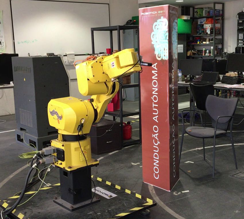
Sensors 2020, 20, 4331                                                                                2 of 30

aerial vehicles, and the ongoing fourth industrial revolution are clear examples of scientific and
commercial drivers for this particular domain of research. We consider as an example of the potential
value of the application of smart autonomous exploration techniques the case of the often refereed
Industry 4.0 movement [1], where Cyber-Physical Production Systems (CPPS) such as autonomous
robotic systems are helping companies to cope with acute alterations in production and business
paradigms [2], frequently needing to operate in highly unstructured and dynamic environments [3].
As a direct result, spatial exploration and object recognition by robotic systems is a key part of many
industry-wide applications and services. Despite being increasingly efficient, this recognition is often
based on the processing of information collected at a single moment, such as images or point clouds.
Thus, most implementations assume that the object recognition process is static, rather than dynamic.
To make this process dynamic, a system needs to have some kind of exploration abilities, i.e., being
able to search and discover information about a given goal.
      The increasingly more dynamic and smart implementations will force a paradigm shift in the field
of exploration by intelligent systems, since these give a new level of adaptability to novel automation
tasks that, at this point, are not possible. These implementations can range from smarter bin-picking,
reconstructing the scene at each iteration for better adaptation, to a system that collaborates with
humans, detecting when something has been repositioned or removed from its working space, and
reacting accordingly. For this shift to be feasible, the new solutions need to be at least as reliable, fast,
and secure as is already standard in today’s industry.
      The ability to explore a new environment, quickly and efficiently, developed to increase our
survival skills, is intrinsic to humans [4]. Our eyes evolved to catch the tiniest of details and our brains
got smarter in understanding the environment and processing it to evaluate the goal, extrapolate the
information gathered, and choose where to move next. This raises the questions: How to give a piece
of hardware that cannot think for itself the human abilities to know what it has and has not already
seen? How to know where it should observe the scene next to gather the newest information available?
      Exploration is the process by which novel information is acquired. In the context of spatial
exploration, the information that is gathered concerns the state of occupancy of the several portions
of the scene. Thus, the goal of scene exploration is to measure the state of occupancy of the
maximum possible regions of the scene. An exploration system requires the ability to conduct active
perception, i.e., to deliberately change the point of view of the sensor with which it observes the scene.
An intelligent exploration system should analyze the current knowledge it has about the scene and,
based on this information, estimate the next point of view to which it should move. This is what we
refer to as NBV. The NBV is selected based (most often solely) on the amount of information it is
estimated it will provide. This exploration step is then repeated until a termination criterion is met.
Common termination criteria are the mission time, the knowledge about a scene, the lack of progress
in the last set of exploration steps, among others.
      As described above, the explorer system must contain a representation of the occupancy of the
different portions of the scene. Furthermore, this representation must be adaptive, in the sense that new
sensor measurements must be integrated into the existing representation. With such a representation it
is then possible to address the problem of selecting the next best view. However, taken at face value,
the problem of finding the best view is a cumbersome one because the set of possible next views is
infinite. The solution for this is to create a finite set of views, where each is tested to estimate the
information it should generate if selected. These views are often randomly generated. The number
of possible views combined with the complexity of the test conducted for each view will define the
computational efficiency of the approach. Within preset time boundaries, the goal is to assess as many
views as possible. One way to address this problem is to create efficient yet accurate assessment
methodologies. Another is to make sure the views which are generated are feasible and plausible.
Feasible because they are within reach of the explorer system, and plausible because they are aimed at
(observing) the volume that is to be explored. This is done with a conditioned randomized procedure.
Sensors 2020, 20, 4331                                                                               3 of 30

Without it, it would be likely that there are several of the generated views that would be unreachable
by the system, or even reachable but not looking at the region of interest.
     All these issues are tackled in this paper. As such, our contributions are the following:

•     To make use of an efficient and updatable scene representation, i.e., OctoMap;
•     To design a generator of plausible and feasible possible viewpoints, which increases the quality
      of the viewpoints that are tested, thus improving the quality of the exploration;
•     To proposed a viewpoint evaluation methodology which sorts the voxels for which rays are cast,
      which enables the algorithm to skip a great number of tests and run very efficiently, thus allowing
      for more viewpoints to be tested for the same available time;
•     To provide extensive results in which the automatic exploration system is categorized in terms of
      the efficiency of exploration, and compared against human explorers.

      The developed method was used to reconstruct a couple of scenarios to assess repeatability.
Also, it was tested against humans, using the part of the tools created during the development of
the autonomous system, to infer if it was advantageous or not to use this exploration methodology.
Furthermore, an industrial prototype application on the scope of a European-funded research initiative
was considering, attesting to the potential applicability of this solution to address some of the
aforementioned contemporary industrial challenges in the domain of autonomous exploration.
      The remainder of this document is divided into four additional sections: In Section 2, a theoretical
overview of some of the concepts addressed by this work as well as several comparable approaches are
presented, emphasizing their strengths and shortcomings. Section 3 presents the proposed approach,
detailing the methodology, roadblocks, and solutions developed to accomplish the enlisted objectives
of this work. This includes the manipulator’s configuration to accept external commands, the mounting
and calibration of the camera, and the exploration algorithms. In Section 4, the authors introduce two
case studies and an industrial prototype application where the developed work is tested, following a
comparison between the autonomous system and several humans’ abilities to explore a given scene.
Still in this section, plausible implementations and further improvements are discussed. Finally,
in Section 5, conclusions are outlined and future work topics are discussed.

2. State of the Art

2.1. Spatial Data Representation
     A fundamental step in empowering autonomous systems to operate in unstructured and
dynamic environments is to gather information to allow evaluation of their surrounding environment.
Point clouds are one of the most common forms of 3D data acquisition. Although they can be easily
acquired, with low-cost sensors that have decent performance, especially at close range [5], this raw
data can easily become hard to process due to the sheer amount of information when considering large
environments. To solve this drawback various methods exist. What these methods try to accomplish is
merging some of the points in the cloud, losing as little information as possible.
     One approach is to create a 2D grid representation of the surroundings, where each cell also
contains a value, typically the possibility of the grid being occupied [6] or height [7]. This last form of
3D representation is referenced as elevation maps. Elevation maps can be classified as 2.5D models
because they have the 2D position information of each cell, which in turn contains a corresponding
height value. This height value is obtainable by various methods. One of the simplest is averaging
the height coordinate of all points falling inside a given cell. The biggest advantage is the filtering of
outlier measurements, but this also leads to the inability of capturing overhanging structures (like
bridges, for example), according to [8].
     To overcome this inability [9] developed the extended elevation map. The indicated approach can
find gaps by analyzing the variance of the height of all measurements in a given cell. If this variance
exceeds a defined threshold, the algorithm checks if this set of points contains a gap that is higher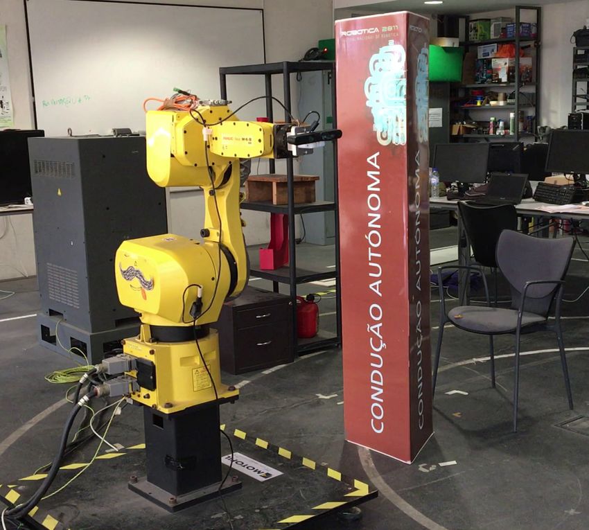
Sensors 2020, 20, 4331                                                                                4 of 30

than the robot they used for testing. If so, the area under the overhanging structure can be properly
represented by ignoring the points above the lowest surface.
      Although the extended elevation maps bring improvements to this type of representation,
its applicability is limited to applications requesting only terrain-like representation. This is a
major issue in the scope of this work since a truly 3D representation is needed. For example, if the
environment that we want to explore only contains a table, using standard elevation maps would give
a fully occupied volume below the table. On the other hand, an extended elevation map would not
properly represent the tabletop, not treating it as occupied.
      That being said, some other methods also use the same philosophy of dividing the space into
a 3D grid, called voxel grids [10]. A voxel grid is generated when the scene is divided into several,
recursively smaller, cubic volumes, usually called voxels (hence the name voxel grid). This division
translates the continuous nature of the world to a discrete interpretation. To represent the scene,
each voxel can have one of three different states: free, occupied, or unknown. In a newly generated
voxel grid, all cells (i.e., voxels) start as unknown, since no information has been gathered yet. When a
point cloud is received, ray-casting from the camera pose to the data points is performed. Ray-casting
consists of connecting the camera position and a point of the cloud with a straight line [11]. Then, in all
voxels that are passed through by a ray we assume that they do not contain an obstacle (i.e., there is
not the acquisition of a point) and so, are identified as free. If, in contrast, a point is sensed inside a
voxel, it is considered to be occupied. This is the core of how states are defined but, in practice, for a
voxel to be considered occupied it must contain more than a given number of points. The opposite
needs to be true for a cell to be free.
      By expanding the concept of grid to a volumetric representation, voxel grids can, as accurate as
its resolution (the size of a voxel side), reconstruct overhanging structures and virtually any object.
Yet they are not a feasible solution as they lack a fundamental characteristic needed for this work,
updatability. In voxel grids, once a voxel state is defined, it cannot be changed. This prevents the
addition of new information (for example, by viewing by a different pose) to the reconstruction.
Furthermore, the resolution is fixed, compromising efficiency, especially in cases that need a large
voxel grid with fine resolution.
      Yet, even with these drawbacks, voxel grids lay the foundations for OcTrees [12], which deal
with multiple resolutions within the same volumetric representation. Building upon the voxel grid
methodology, OcTrees are a data structure that divides the pretended portion of the world into voxels
but allows those voxels to have different sizes. In an OcTree, each voxel can be divided into eight
smaller ones, until the minimum set resolution is reached [13]. It is this subdividing property of the
voxels that establishes a recursive hierarchy between them [14]. This resolution multiplicity means
that some portions of the space that have equal state (this is, are free or occupied) can be agglomerated
in one larger voxel. This is called pruning. Pruning occurs when all eight leaves (the nodes of the
OcTree that have no children) of a node are of the same type, so they can be cut off, requesting lesser
memory and resources, which improves efficiency.
      Recursing through the OcTree structure allows most of the information of the inner nodes to
be obtained. For example, the depth of a node can be calculated by adding one to its parent depth.
A similar thought can be traced to the position and size of a node. To optimize memory efficiency, any
information that is computable by traversing the tree can be omitted [15]. Furthermore, in cases where
the mapping is performed for large spaces and high resolutions are required, voxel interpolation
methods can be applied to obtain similar results with lower memory consumption and better
framerates [16].
      Although the efficiency issue of voxel grids is solved, OcTree still lacks updatability that by itself,
is already a challenge, requesting a criterion which leads to a voxel changing its state. In a voxel grid,
each voxel can store a value that defines if it is free or occupied. In the case where that measurement
was not taken, the voxel encounters itself in an unknown state. In a probabilistic voxel space, its value
ends up being the probability of a voxel being occupied. Since we are dealing with probabilities,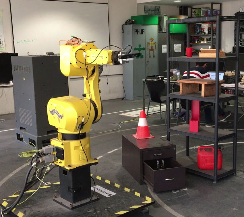
Sensors 2020, 20, 4331                                                                               5 of 30

a new measure of the environment can be integrated to update those probabilities. With a changing
occupancy value comes the possibility of a voxel changing its state. There are several ways in which
the integration of a new measure can occur.
      OctoMap [17] manages this process using the log-odds of a voxel being occupied instead of the
direct probability value. This causes the substitution of multiplications by sums, achieving a more
efficient algorithm. In the works of [18], the OctoMap voxel space update procedure is improved in
a way that now considers reflections. Using the MURIEL method [19], this approach adds a parcel
to the overall probability of a voxel being occupied that is referent to measures in specular surfaces.
In addition to this change, ref. [18] also uses Dynamic Multiple-OcTree Discretionary Data Space.
This structure allows the use of multiple octrees for discretizing the space.
      OctoMap delivers an efficient data structure based on OcTrees that enables multi-resolution
mapping, which can be exploited by the exploration algorithms [20]. Using probabilistic occupancy
estimation, this approach can represent volumetric models that include free and unknown areas,
which are not strictly set. As proven by [18], OctoMap still has room for improvements such as being
able to consider reflections and to be based on the actual sensor model. Yet it is the most efficient and
reliable 3D reconstruction solution currently available.

2.2. Intelligent Spatial Data Acquisition
      With a found way to accurately represent the environment and its changes, the next logical
step is to feed the map with measurements. These measurements could be taken by putting the
object/scenario on a rotating platform [21] or by moving the camera through a set of fixed waypoints.
Neither of these solutions is very good in terms of adaptability to the environment, being useful only
in a few situations.
      An intelligent system needs to adapt to anything that is presented to it, deciding by itself to where
it should move the camera, to obtain the maximum possible information about the scene. In some
particular cases, part of the scene cannot be observed, for example, a box with all six sides closed.
The system must understand when it has found a situation like this and give the reconstruction process
as completed.
      In [22] the goal was to find a sequence of views that lead to the minimum time until the object
was found. To achieve this, they determine the ratio between the probability to completely find the
target—with a given pose—and the transition time that takes to get there. With their utility function,
the planner favored three situations: (i) locations that are closer to the previous position, (ii) locations
where the probability of finding the object is very high or (iii) a combination of the previous two points.
The innovation in this approach is that they plan several steps and, after each pose evaluation, the list
of poses that are intended to be visited is updated. By using, as the authors describe, “the probability
to find a target with observation after having already seen the sequence they assume that all possible
positions are determined by sampling, and so the problem is not only to generate them but also to
choose which ones to visit and in what sequence” [23].
      Since replanning occurs in every pose, a condition to stop the planning procedure must exist.
In [22] the planning ends when the probability of finding the unknown voxels, by adding a new
pose, falls below a user-given threshold. The described methodology worked very well on the
authors’ experiments. Yet, taking into account that this work will use a robotic manipulator (that
compared with the PR2 robot is not able to move as freely) the moving time component used in their
approach will not reveal a great significance.
      When [24] tackled the problem of semantic understanding of a kitchen’s environment, they used a
2D projection of the fringe voxels on the ground plane allied to the entropy of the space within the view
frustum (i.e., the region of space that is within the Field of View (FOV) of the camera). This entropy
is the measurement of how many voxels in different states are possibly detectable by the pose being
evaluated. The more different they are, the higher the entropy will be. On the other hand, fringe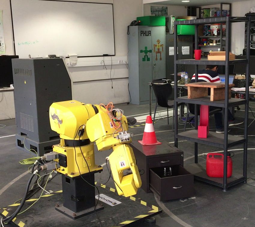
Sensors 2020, 20, 4331                                                                                6 of 30

voxels are considered windows to the unexplored space because they are marked as free but have
unknown neighbors.
      First, it is necessary to introduce the concept of a cost map. A cost map is a data structure able to
represent places in a grid where it is or is not safe for a robot to move in. What [24] does is to create
two separate cost maps for the fringe (CF ) and occupied (CO ) voxels and then combine those values.
The combination makes each cell store the minimum value between CF and CO (representing the
lowest risk of collision). Now, choosing the maximum value from the combined cost map they achieve
a pose from which as many fringes and occupied voxels are observed, with little risk of collision. It is
necessary to observe several occupied voxels because there is a need to achieve a 50% overlap with this
new view and the already created map. In [24] moving expenses were not considered, which meets the
intended for this work, but further adds a new type of voxel (fringe), which makes sense in the large
rooms they focused and, furthermore, removes the need to evaluate occlusions. For object exploration,
these fringe voxels increase the complexity of the system in a direction that will not produce any
significant advantage. We need, in each new pose, to evaluate the largest possible number of unknown
voxels, whether they are close to free space or not.
      An alternative is to estimate the score of a pose by the volume it could reveal. As with what [24]
called fringe voxels, ref. [25] define frontier cells as the ones that are known to be free and are
neighboring any unknown cell. Their goal is to remove all unexplored volume, called voids. For each
frontier cell, a set of utility vectors are generated. These vectors contain information about the position
of this cell, the direction from the center of the void to the cell, and the expected score value from
that cell (i.e., the total volume of the cells that are intercepted with ray tracing, from the center of
the frontier cell to the center of the void). For each free cell that is intersected by a utility vector, ray
tracing is performed with its direction, and the utility score stored. Of all these viewpoints, those who
are outside the robot’s workspace are pruned and the remaining are sorted by their util (c) values for
computing valid sensor configurations. In other words, this means—after sorting the viewpoints by
their score—sampling some valid camera orientations and perform, again, ray tracing. After a given
number of poses has been computed, the next best sensor configuration is the one that has the highest
utility score (i.e., allows the observation of most volume). The recognition process terminates when
the last view utility is null.
      Another possibility to choose between the sampled poses is not by their total information gain
but, instead, ranking them compared to each other. With this goal, ref. [26] proposes a utility function
that compresses the information gain and robot movement costs of a given view with the cumulative
information gains and movement costs of all view candidates. When a pose gives the maximum
relative information gain with the minimum relative cost, the authors consider that they achieved
the NBV. When the highest expected information gain of a view falls below a defined threshold the
reconstruction is completed. Until this point, the utility functions are composed of a small number of
inputs (one to two), but larger equations are possible.

2.3. 3D Object Reconstruction and Scene Exploration
      Trying to get an algorithm that was optimal for motion planning in 3D object
reconstruction, ref. [27] came up with the goal to maximize a utility function composed by four
distinct inputs: (i) position, related to the collision detection, (ii) registration, a measurement of
overlap between views, (iii) surface, which evaluates the newly discovered surface, and (iv) distance,
to penalize the longer paths.
      If a position requires a path that enters in collision with the environment, the position portion
of the equation is set to zero, eliminating that candidate. The registration part is evaluated as one
if the overlap portion of the new view is above a given threshold, or zero otherwise. Next comes
the first non-binary value, related to the new surface measured, that gives the number of unknown
voxels sensed with that view, normalized by the amount of the total unknown voxels in the workspace.
The final value is inversely proportional to both translation and orientation movements since the goal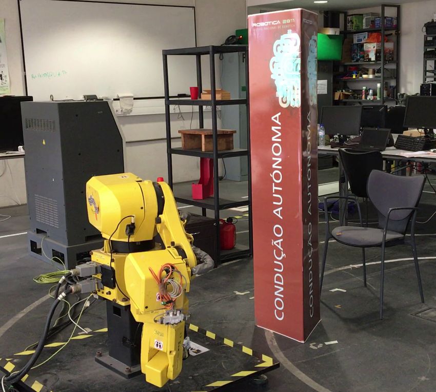
Sensors 2020, 20, 4331                                                                               7 of 30

is to maximize, the smaller the length, the greater this value will be. To stop the reconstruction process,
a condition is used which is based on the number of sensing operations needed to have a certain
confidence of having sensed a portion of the object.
      This creates two scenarios, the first in which the percentage of voxels inside the object is known a
priori and the number of sensing operations is calculated once, or the second one where that value is
unknown and so, this number is recalculated in every cycle. When the sensed portion does not change
within this amount of operations, the task is considered to be over with the requested certainty.
      One thing that has been missing in all the described utility functions is a parcel specifically
dedicated to the modelling part of the problem. An introduction to this methodology is performed
by [28], in which two goals exist, the full exploration of the scene and the modelling of it with decent
surface quality. These two goals gain or lose relevance in the output of the utility function based on
the number of scans performed, making the best NBV the one which gives the most entropy reduction
with the most surface quality. In their respective setups, both [29] and [28] use an RGB-D camera
combined with a laser striper. Allied, these devices combine the faster and completer overview of
the scene provided by the RGD-D camera with the superior surface quality reconstruction from the
laser striper. In the latter case, initially it is wanted a rough but broad mesh of the object but, later,
the quality of that mesh begins to matter the most. To perform this change, a transition value is chosen.
This value comes in the form of a weight, based on the number of scans already performed of the scene.
      In [28] the stopping criteria were more recognition oriented, so the process was established to
end when, at least, 75% of the object was modelled. Yet, the end of the process can be reached when
there is already enough mesh coverage and relative point density. If neither is reached, ref. [18] also
implement a maximum number of scans criteria. They also introduce a method for switching from
generating candidate poses to rescanning (in their case, rescanning holes in the mesh) if the increase in
coverage of one scan compared to its previous is less than 1%.
      All the methods already described lay in predefined evaluation functions and human set
threshold values. These methods are considered to be a more classical approach to solve a
computational task. Currently, the trend to solve such tasks is to use neural networks and provide
systems with artificial intelligence. These systems can be taught by analyzing examples, like manually
labelled data. With the spreading of neural networks and artificial intelligence, the usage of this new
and powerful methods has already been accomplished in some particular situations.
      Remembering that each voxel stores a probability value of being occupied, ref. [30] uses a utility
score function that defines the decrease in uncertainty of surface voxels (voxels that intersect the
surface of the object being reconstructed) when a new measurement is added. The goal here is to
predict this value without accessing the ground truth map. Using a ConvNet architecture, trained
with photo-realistic scenes from Epic Game’s Unreal game engine, the 3D scene exploration occurs
in episodes. An episode starts by choosing a random starting position to mark it as free space.
Progressively, at each time step, the set of potential viewpoints is expanded to the neighbors of the
current position, all of them are evaluated and the robot moves to the best one. The authors claim
that their model can explore new scenes other than the training data but is dependent on the voxel
distribution of the said data. They also do not contemplate moving objects in the scene and are bound
by the resolutions and mapping parameters of the training data.

2.4. Contributions beyond the State of the Art
     The proposed approach for solving the problem planned for this work consists of an
adaptation and blend between [25] view-sampling method, ref. [26] utility function and [27] surface
parcel computation. With a set of points representative of where the camera should look seems a good
starting point for the view-sampling procedure, increasing the chance of those pose being plausible.
To be plausible, a pose must have, somewhere in their FOV, at least one unknown voxel expected to
be evaluated. Comparing and ranking those poses against each other makes it possible to introduce
stopping criteria that directly correlates to the first NBV and so, it is expected that in each exploration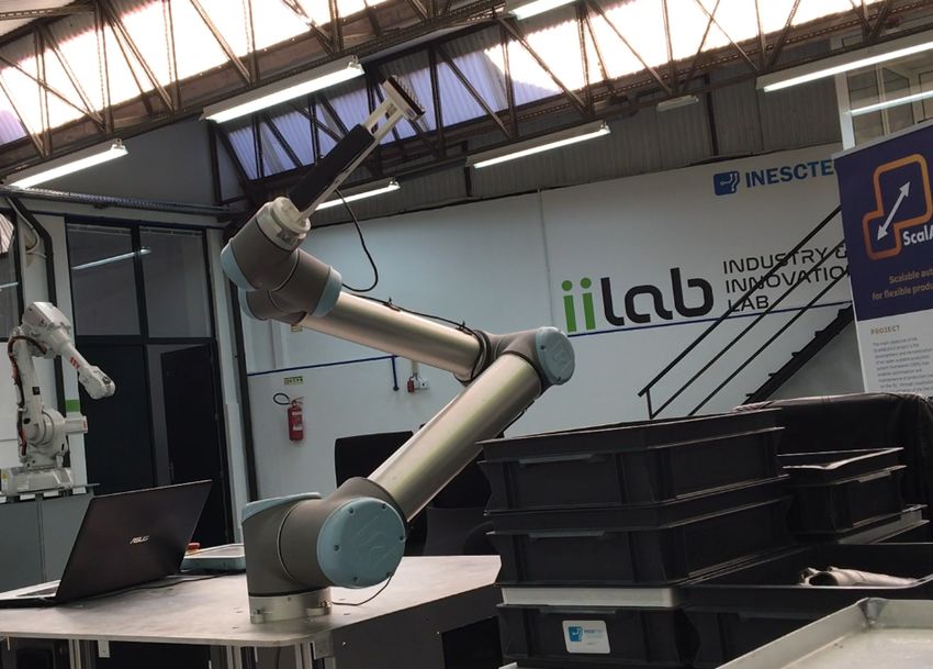
Sensors 2020, 20, 4331                                                                                                     8 of 30

iteration (i.e., the movement of the robot to a new viewing pose) the NBV score always decreases.
The use of neural networks was not considered since their potential in this field has not yet been
proved to introduce advantages that overcome the limitations and, maybe even more relevant, the
time-consuming process of training and evaluating it.
      For the reason that the proposed approach relies on an active perception system [31], after deciding
where the camera should move, a path to get there must be planed. This path cannot enter in collision
with the environment, under the penalty of changing it or causing damage to the hardware. This means
that to correctly plan the path of every element of the autonomous system (in the case of this work, the
3D camera and the robotic manipulator), their relative positions must be known. Eventually, we could
also take advantage of this path to enforce on it a subset of goals poses that would increase even further
the amount of collected information [32].

3. Proposed Approach
      The ability to conduct autonomous exploration requires an accurately calibrated robotic system
so that the system can anticipate the pose of the in-hand sensor as a function of the manipulator’s
joint configuration. Also, a criterion for the adequate selection of the NBV is required, as a means for
the system to plan the most adequate motion to explore the scene. In this sense, the NBV is defined as
the camera pose which maximizes the amount of new information gathered about the scene, which is
dependent on the current state of the reconstruction of the environment.
      To address the first requirement, a calibrated system, a hand-in-eye calibration war performed.
This procedure returns the geometric transformation between the manipulator’s end-effector link
and the camera sensor link and works by capturing multiple and representative views of a
calibration pattern. The ARUCO / VISP Hand-Eye Calibration (https://github.com/jhu-lcsr/aruco_
hand_eye (accessed on 16 March 2019)) provides an easy way to implement Aruco-based extrinsic
calibration to the system.
      Providing a way to explore a given volume autonomously is the overall objective of this work.
To do so, the architecture depicted in Figure 1 is proposed. This architecture allows for a fully
autonomous exploration that always guarantees the manipulator’s movement to the pose estimated to
give the most information gain and which it can plan for. The next subsections will present in detail
the functionalities described in the proposed architecture.

                                                                                                              No

             Generate    Evaluate       All Poses Yes    Choose     Plan Robot    Planning Yes   Move    Threshold   Yes
 START                                                                                                                     END
              Pose        Pose         Generated?       Best Pose      Path      Succeded?       Robot   Reached?

                                            No                                          No
                                                                                 Choose Next
                                                                                  Best Pose

                                    Figure 1. Flowchart of the full exploration algorithm.

3.1. Defining the Exploration Volume
      The objective of the exploration may not be to explore the entire room but, most often, just a small
portion of it. In addition to this, it is intended that these exploration systems operate online, and a
delimitation of the volume to be explored is an effective way of speeding up the process. To address
this, we propose the concept of exploration volume, which is intended to be explored. In other words,
the system considers that there is no information gain in observations outside this volume.
      Notice that this cannot be done just by discarding the points outside the exploration volume,
because the construction of an OcTree map builds not only from the points themselves but also from the
ray that goes from the sensor to that point. A point that lies outside the exploration volume may still
create a ray that is important to build the representation inside the exploration volume. The solution is
to define a second, larger region named point cloud filter volume. In these experiments, a region five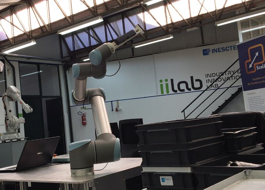
Sensors 2020, 20, 4331                                                                                           9 of 30

times larger than the exploration volume was used. This value was empirically obtained as the best
compromise between memory usage and the performance of the map reconstruction. Points outside
this larger region are then discarded. Figure 2 shows an example which explains the purpose of the
point cloud filter volume. Since in Figure 2a the exploration and filter lines are coincident, the beam
bounces back outside the filter, disabling its registration, making it impossible to mark the black voxel
as free. On the other hand, in Figure 2b, the point is detected since it is inside the point cloud filter,
allowing the unveiling of the black voxel free state.

                            (a)                                                        (b)
      Figure 2. Exploration volume vs. point cloud filter volume: (a) coincident and since the ray is reflected
      outside the point cloud filter volume, it is impossible to know in which state the black voxel is: (b) point
      cloud filter volume larger than exploration volume, the point is registered and the state of the voxel
      is known.

     This solution ensures two things: the OctoMap does not become very large and detailed in
unimportant regions and that there is not an excessive amount of information filtered out. Figure 3
displays the complete filtering procedure.

      Figure 3. Definition of the point cloud filter volume (each side is two times bigger than those of the
      exploration volume). Exploration volume (orange represents unknown space, red occupied space.
      Free space hidden for visualization purposes). Blue lines mark the boundaries of the point cloud filter
      volume. Filtered point cloud also visible.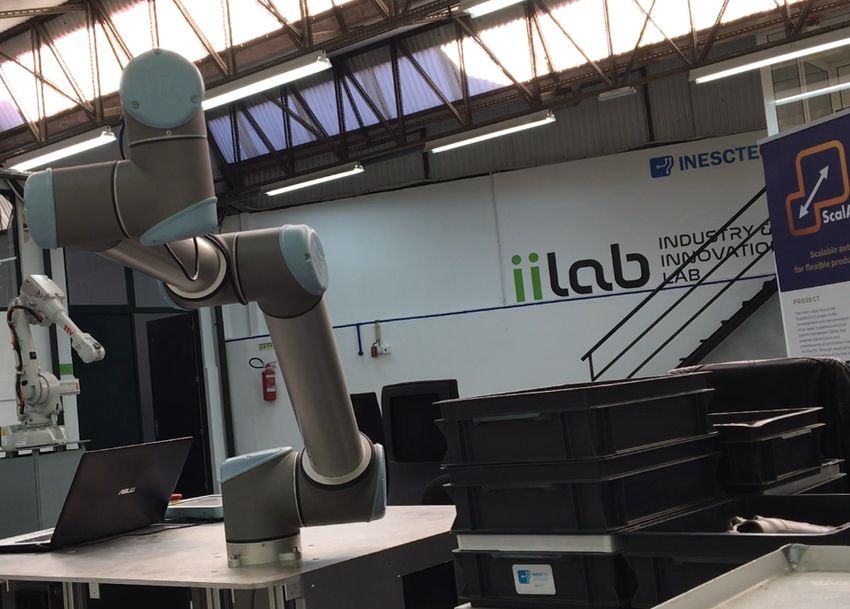
Sensors 2020, 20, 4331                                                                                   10 of 30

3.2. Finding Unknown Space
     Having developed an effective way of constructing online an OcTree representation of a volume
to be explored, the goal now is to assess which regions in that volume have not yet been explored.
Notice that ocTrees do not store information about unknown voxels explicitly. To extract this
information, we iterate through all voxels of the OcTree and verify if their state remains undefined.
     It is also important to group the set of unknown voxels into spatially connected clusters.
The reason for having these clusters of unknown space is to be able to generate plausible sensor
poses as is detailed in Section 3.3. Clusters are built by iterating through all the centers of the unknown
voxels, and testing if the distance to the neighbors is within a predefined distance (in this case, just over
the double of the OctoMap’s resolution). An iterative procedure forms clusters that grow until all the
neighbor voxel centers are too distant. The procedure is similar to a flood fill or watershed algorithm
in image processing. The result of the clustering procedure can be observed in Figure 4a. For each
cluster of unknown voxels we compute the center of mass of its constituent voxels: see Figure 4b for
the centroids that correspond to the clusters of Figure 4a.

                              (a)                                               (b)
      Figure 4. Example of ten clusters found after an exploration iteration. (a) Point clouds (points are
      the center points of the unknown voxels) that define each cluster. (b) Respective clusters centroids.
      Different colors represent different clusters.

3.3. View-Sampling
      View-sampling is the process by which several views, i.e., camera poses, are generated. Notice that
the goal is to generate a set of random camera poses and to select the best one from that set. In this
context, the best view would be the one that maximizes the information gain. To select the best view,
each pose must be evaluated. This evaluation process is time-consuming, which in turn restricts the
number of evaluated views per exploration loop.
      Given this, it is nonsensical to generate (and evaluate) entirely random views, since a significant
number of these would not be able to gather information about the exploration volume. On the other
hand, it is important to maintain an ingredient of randomness in the generation of the views, so that it
is virtually possible to visit any view. To address this, we propose a procedure to which we refer to as
conditional randomized view-sampling. Each view is a sensor pose in world coordinates. The process
divides the views into two components: position and orientation.
Sensors 2020, 20, 4331 11 of 30
The position components are randomly sampled within the reach of the robotic manipulator
using MoveIt [33]. To prevent poses where the manipulator itself occluded the exploration volume,
the position generation is also limited to the front hemisphere of the working space. This first stage
generates a set of incomplete sensor poses that contain only the translation components. For reaching
those poses, an orientation component is generated. The center of observation, i.e., the center of
the unknown voxels cluster to which each sensor pose is associated with, is used to generate the
orientation. Using the position of the pose and the center of observation a z versor (the direction which
the camera will look at) is computed coincident to the line that unites both points. The y versor comes
from the cross product between the z versor and a random vector and the x versor is also the cross
product between the already defined z and y versors. Figure 5 gives an example of a set of generated
poses following this procedure.
Figure 5. Example of 50 poses generated using a conditional randomized approach, bounded by the
systems reach. In this case, there is a single unknown voxel cluster, to which all sampled poses are
pointing at. Unknown space is hidden for better visualization. Voxels in blue are the ones expected to
be evaluated based on the best pose of those sampled, colored as green.
This method gives a solution to produce a set of plausible poses. To decide which to visit we need
to score and rank them all. The first request to give a score to a pose is knowing how much unknown
voxels it unveils. This procedure takes into account the reach of the robotic system, i.e., if the system
can position the camera at the set of plausible poses.
View-sampling requires information about the center of the clusters, so they acquire the best
orientation. The total number of poses is a parameter and the algorithm evenly distributes that quantity
by all the found clusters, as in Equation (1),
Nposes
ppc = round , (1)
Nclusters
where ppc is the number of poses per cluster, Nposes and Nclusters are, respectively, the number of total
desired poses and found clusters. The advantage of this method is that the total number of poses
is independent of the amount of clusters found, allowing for a more stable time consumption per
exploration iteration, when compared to if the amount of poses was set for each cluster found.
3.4. Generated Poses Evaluation
The next step is to be able to evaluate each of the previously generated poses. The evaluation of
these poses is based on the estimated amount of volume that is (or can be) observed by the robot when
positioned on that pose. As noted before, we are simply estimating the volume that may be discovered
by a new pose. This is an estimate since it is not possible to be sure if some regions of the yet to be seen
volume will be occluded.
To estimate the volume that may be observed, we propose an algorithm based on ray-casting
driven by the centers of the unknown voxels that lie inside the camera frustum. Figure 5 also shows anSensors 2020, 20, 4331 12 of 30
example evaluation of a pose where the voxels expected to be known, if the robot is placed on that
pose, are colored blue. A method to retrieve this information is introduced in the following subsection.
3.5. Voxel-Based Ray-Casting
This method starts the ray-casting on the unknown voxels instead of on the pose. This not only
has the potential to give higher resolution to locals with more unknown voxels but, also, significantly
decreases the number of rays to be cast. If we start the casting from the furthest voxel to the closest
(relative to the pose to be evaluated) there is a high chance that the first rays intersect a large number
of voxels. Assuming that in this evaluation, a voxel only needs to be visited once for its state to be
defined, there is no need to cast a ray again for those voxels (that have already been intercepted),
eliminating them from the queue, reducing the overall rays to be cast.
After computing the central point of all unknown voxels, we start by defining the set of those that
lay within the frustum, since only these have the potential to be discovered. These points, and their
corresponding voxels, are sorted by distance to the pose being evaluated. Starting from the furthest
voxel, the direction from the pose to its central point is computed. This direction is used to cast a ray
that if there is not any occlusion, will pass through the voxel. All the voxels that are intercepted by this
ray will not be visited again, since we already have the confidence that at least one ray will hit them.
In the case where the ray ends in an occupied voxel, it is necessary to take into account the voxels that
are occluded. Therefore, following the same direction, from this occupied voxel until the end of the
frustum, those voxels that would be intercepted by this hypothetical ray will not be visited any time
and neither be assumed to be discovered. Then, for the next furthest voxel that has not been visited
yet, the process repeats itself until all the volume is evaluated. Algorithm 1 describes this process.
Figure 6 represents the visual outcome of this algorithm, where is visible the casted rays
(gray lines), the occupied (red), free (green), unknown (orange) and expected to be known (blue)
voxels, as well the camera frustum.
(a) (b) (c)
(d) (e) (f)
Figure 6. Evaluated pose. This figure shows the beams passing the free space (green) and stopping
when they hit an occupied voxel (red). The voxels that potentially will be known are marked in blue.
In (a), everything is shown. In (b), it is visible the unknown, occupied, and expected to be known
volumes. (c) is similar to (b), but the unknown volume was removed and the free added. In (d), only
the occupied and expected to be known volumes are showing. In (e,f), the expected to be known and
occupied volumes are shown.Sensors 2020, 20, 4331 13 of 30
Algorithm 1: Voxel-Based Ray-Casting.
Input: pose, near_plane_distance
Output: list of voxels expected to be known
get the voxel centers that lay within the camera’s frustum;
foreach voxel inside frustum do
get the distance to camera;
end
sorted_voxels ←sort voxels from furthest to closest to the pose;
foreach voxel ∈ sorted_voxels do
if voxel is marked to be visited then
direction ←compute direction from pose’s origin to voxel’s center;
ray_endpoint ←cast ray from pose’s origin, with computed direction;
ray_keys ←get the keys of all voxels passed through by the casted ray until reaching
ray_endpoint;
foreach key ∈ ray_keys do
key_voxel ←get voxel corresponding to that key;
distance ←compute distance from pose’s origin to key_voxel;
if distance > near_plane_distance & key_voxel is unknown then
register the voxel according to its order of passing;
set voxel to not be visited again;
end
if key_voxel is occupied then
set all voxels after key_voxel to not be visited;
end
end
end
end
Now we want to rank the poses against each other. The metric implemented to do so, i.e., the
formulation that gives a score to a pose, is based on this assessed unknown volume to be discovered.
3.6. Pose Scoring
To rank all the poses, a term of comparison must be set. In this work, when estimating how many
voxels a pose will evaluate, we expressed this value as a volume. Then, it becomes straightforward that
the term of comparison should also be a volume. As referred in Algorithm 1, the order in which the
voxels are intersected is a useful information. The first voxel which is intersected is always assessed.
As other voxels which lie behind the first (along the casted ray) will be visible or not depending on
whether an occupied voxel surges in front of it.
Since the quantities of voxels that are the first to be intercepted by a given ray, n f irst , and that
are intercepted by a ray but have an unknown voxel between them and the evaluated pose, n posterior ,
are known, as well as the OctoMap’s resolution, a weight w ∈ [0, 1] can be set to give less relevance to
the voxels which are uncertain to actually be observed,
(n f irst + n posterior × w) × resolution3
score = (2)
volumeouter + volumeinner × w
where volumeouter is the aggregated volume of all voxels that have at least one face exposed, and the
volumeinner is the volume of all voxels that have all their faces connected to another unknown voxel.
Both volumes are computed before the exploration begins and have the objective of normalizing the
pose’s revealed volume similarly as estimated.Sensors 2020, 20, 4331 14 of 30
Scoring a pose is also useful in the sense that provides stopping criteria for the process.
When a set of poses are sampled and the best of their scores does not get above a given threshold
(i.e., max(scorek ) < threshold, k ∈ Nn poses , where n poses is the defined maximum number of poses to be
sampled), that pose is still visited since it was evaluated but will be the last given that from this pose
onward, the information gain will surely be below the pretended value. This can occur by two factors:
either all the unknown volume has actually become known or the voxels that remain unknown are in
unreachable places. Having gathered the desired, possible, information about the previously unknown
scene, the process finishes successfully.
4. Results
This chapter presents results of the developed system and, when opportune, discuss its limitations,
applications and possible improvements in a future continuation. The first topic to discuss is the
functionality and autonomous capabilities of the developed system and for that three test scenarios
will be introduced. These scenarios intend to show real-world applications. In the first two scenarios
were at Laboratório de Automação e Robótica—University of Aveiro (LAR-UA) built to challenge
the system, posing two different challenges. In the third scenario, we demonstrate a prototype of an
industrial application scenario where this autonomous exploration system would allow the unveiling
of parts inside containers for further manipulation in bin-picking operations. The industrial scenario
was considered on the scope of the H2020 FASTEN R&D project [34] and required an alteration on the
hardware architecture employed.
4.1. Test Scenario 1: Shelf and Cabinet
This first scenario consisted of a cabinet that has a shelf behind it. The shelf has some objects
on the shelves to generate occlusions, and, on the cabinet, one of the drawers is semi-open, and
contains an object inside, creating a volume that cannot be seen and other that can only be visualized
from a narrow set of viewpoints. The complete scenario can be seen in the right column of Figure 7.
Figure 7 describes the exploration process for this scenario, taking six iterations (only three shown)
and sampling 150 poses for each, with the finest map resolution defined at 40 mm. The exploration
volume is 3.238 m3 and the reconstruction ended when the NBV had a score of less than 0.1%. For this
reconstruction was defined that the finest resolution was 25 mm since it gave the most details without
a big compromise in performance. This resolution allows the capture of finer details.
In the first iteration (before the movement of the robot, Figure 7a) a large amount of volume is
expected to be observed, due to no information about the scene. In Figure 7b, it is discernible the
exclusion of some voxels in the expected volume to be known, as a result of the occlusion created by
the traffic cone. Yet, after the pose was reached, we can see that the refereed voxels have in fact been
evaluated (in this case, as free) in conjunction with some other in front of the cabinet. This happens
because of the path taken by the camera. While moving, the camera is continuously sensing what is
inside its FOV, sometimes providing information where it was not expected to be collected, depending
on the path travelled. This factor was not taken into account during the evaluation of poses because it
would request a great amount of computational power to evaluate all steps of the path (these steps can
add up, surpassing the hundreds).
This iteration also demonstrates a characteristic movement of the robot, going from right to left
to access the state of the voxels positioned where the camera has not looked up until this moment.
This NBV was oriented to look towards the bigger cluster in the front right of the exploration volume.
Nevertheless, some voxels belonging to different clusters are also expected to be visible and within the
FOV, which increases the score of that pose. Because some were behind a solid obstacle (yet unmapped)
not all of them were actually observed. In the next few iterations, the robot bounces right and left
gaining information about a decreasingly unknown volume until the stop criteria are met. At the end
of the process is visible the almost absence of unknown volumes (Figure 7c), which has been evaluated
to be free or occupied.Sensors 2020, 20, 4331 15 of 30
(a)
(b)
(c)
Figure 7. A sequence of iterations for the complete reconstruction of the shelf and cabinet scene. On the
left are all the possible poses (the more blue the better score, and the redder the worst), the chosen NBV
(in green and bigger), the unknown voxels in orange and the voxels expected to be known on blue.
In the middle is what the pose actually improves the model, red voxels are occupied, green represents
the free space. On the right is the actual pose of the robot. (a) shows the first exploration iteration,
(b) the reconstruction improvements of an intermediate iteration and (c) is the result when the process
is concluded.
The shelf and cabinet scenario provided a challenging reconstruction because of its high
complexity, with multiple objects, intricate spaces, and volumes impossible to be seen, requesting from
the robot several demanding poses to achieve its goal. Despite this, it took an average of eight poses to
fulfil the task. The goal for this section was to provide a more qualitative evaluation and demonstrate
how the process unfolds, with the quantitative results being discussed in Section 4.3. This philosophy
will be maintained in this next section, where a new scenario is presented.Sensors 2020, 20, 4331 16 of 30
4.2. Test Scenario 2: Occluded Chair
The previous scenario lacked a big occlusion that would challenge the pose evaluation procedure,
testing its real aptitude to deal with these kinds of challenges. Going even further, the system must be
able to react to an occlusion that is expected to happen and move around it, visiting poses that are
expected to return the biggest possible information, without interacting with the scene, i.e., without
colliding with it.
This new scenario is presented in the right column of Figure 8, where the chair is visibly occluded
by a tall obstacle with a triangular base. Being this tall forces the robot to look from either side,
disfavoring central positions, while making it impossible—given the reach of the manipulator—to look
inside of said obstacle by its only entry, at the top. The obstacle is also close enough for the robot to
collide with it if no collision checking would be performed.
Two big, unknown, volumes were not sensed in this exploration: behind the chair and inside the
obstacle. The unknown cluster in the rear of the chair exists solely due to the robot’s inability to reach
a pose in which the camera can perceive that volume. Similarly, as already referred, the set of poses
able to unveil the cluster inside the barrier would be in a very high position looking down. However,
even these would not grant a complete evaluation of the said volume since the obstacle is taller than
the FOV of the camera. Therefore, to completely unveil this volume, the robot had to reach a high
position and then, probably, go inside it in a second one. Unfortunately, these poses and movements
are out of the manipulator’s reach.
Another aspect is the poor reconstruction of the back portion of the obstacle, once again explained
by the inclination of the planes. As represented in the previous figure, some voxels, in the same vertical
line, are occupied and others free, when was expected for all of them to be in the same state. The most
plausible explanation lays in the orientation of the walls. Given the reachability of the manipulator,
most of the rays intersecting these voxels would be almost parallel to the barrier, passing through
them without actually hitting the barrier, wrongly setting them as free. Yet, in another pose, possibly
with a higher rotation, these rays actually bounce on the barrier, setting those voxels as occupied.
This uncertainty would explain the high entropy of the reconstruction of those two back barriers.
As discussed when analyzing the reconstruction of the shelf and cabinet scenario, the first NBV
does not contemplate information about occlusions. By chance, in this first iteration (Figure 8a), only
the lower portion of the set is evaluated, requesting a pose capable of sensing the higher portion,
which happens next. After the second exploration iteration, the barrier has already been mapped,
allowing for full occlusion avoidance poses, exactly as happens in Figure 8b, where the robot, almost
all stretched, looks from right to left to reveal the remaining top portion of the exploration volume.
Finally, like in the previous scenario, there is the last iteration where a small number of unknown
voxels are measured to fulfil the end criteria.Sensors 2020, 20, 4331 17 of 30
(a)
(b)
(c)
Figure 8. A sequence of iteration for the complete reconstruction of the occluded chair scenario. On the
left are all the possible poses (the more blue the better score, and the redder the worst), the chosen NBV
(in green and bigger), the unknown voxels in orange and the voxels expected to be known on blue.
In the middle is what the pose actually improves the model, red voxels are occupied, green represents
the free space. On the right is the actual pose of the robot. (a) shows the first exploration iteration,
(b) the reconstruction improvements of an intermediate iteration and (c) is the result when the process
is concluded.
One of the goals when testing with this different scenario was to evaluate how the robot reacted,
and planned, to an object within its reach. Figure 9 illustrates an example case where this happens.
After having reconstructed part of the scene, the robot selected a pose that requested it to move across
the scene but, if taken a straight path, would collide with an object it already knows the existence of.
To avoid it, the camera curves down and inwards in the process, distancing itself from the barrier.
When reached a position where a collision was not expected to occur anymore, an upward path wasSensors 2020, 20, 4331 18 of 30
taken to achieve the goal pose. To achieve this behavior, various path planners are available and in
this work, the one chosen was RRT-Connect [35] since it proved to be the one who allied efficiency,
simplicity and the better interaction with the environment.
Similar to what happened for occlusions, this behavior tends to react better to the obstacles as more
and more knowledge about the environment is gathered. It also gives the insurance of a completely
autonomous exploration by the robot. The ability to generate a model of a new environment, without
changing it with a collision is there, achieving the goal of this work. Accessing if it is advantageous to
use in replacement of a human controlling the manipulator is discussed further ahead in Section 4.5.
(a) (b)
Figure 9. Path taken by the depth optical frame to reach the goal pose, without colliding with the space
already known to be occupied. (a) is the top view and (b) is a perspective view.
4.3. Experimental Analysis of the Autonomous Exploration Performance
In this section, a set of quantitative results is provided. These results compare the technique
adaptation of the algorithm to both scenarios already described. The summary of the physical
characteristics and performance of the algorithm is highlighted in Table 1. For the results that follow
it was requested to the system to reconstruct both prior scenarios—six times each—with stopping
criteria defined at 0.1% (accordingly to Section 3.6) and 40 mm OctoMap resolution. To accomplish
this, 150 poses were sampled by exploration iteration. Table 1 additionally summarizes the statistical
information for each scenario, either the requested number of iterations and also the agglomerated
distance between the visited poses.
Table 1. Statistical results of the explorations in Case Study 1, shelf and cabinet and occluded
chair scenarios.
Number of Total
Exploration Iterations Distance [m]
Scenario
Volume [m³] Standard Standard
Mean Mean
Deviation Deviation
Shelf and Cabinet 3.531 8.00 1.789 8.525 1.084
Occluded Chair 2.140 5.17 0.408 6.365 1.089
It is evident that when the exploration volume diminishes, fewer iterations, and therefore poses,
are required to fully reconstruct the environment. This leads to a shorter travelled distance by the
camera’s depth optical frame, but even so, the dispersion of the travelled distance between poses
remains approximately the same. This means that the algorithm diversifies its poses no matter the
volume to explore, which makes sense considering that this behavior tends to maximize the gain of
information by consecutive iterations. Through measuring both volumes a NBV is expected to revealYou can also read