CEP Discussion Paper No 1620 May 2019 Trade Blocs and Trade Wars during the Interwar Period David S. Jacks Dennis Novy

ISSN 2042-2695

 CEP Discussion Paper No 1620
 May 2019

Trade Blocs and Trade Wars during the
 Interwar Period

 David S. Jacks
 Dennis Novy

Abstract
What precisely were the causes and consequences of the trade wars in the 1930s? Were there perhaps deeper
forces at work in reorienting global trade prior to the outbreak of World War II? And what lessons may this
particular historical episode provide for the present day? To answer these questions, we distinguish between
long-run secular trends in the period from 1920 to 1939 related to the formation of trade blocs (in particular, the
British Commonwealth) and short-run disruptions associated with the trade wars of the 1930s (in particular,
large and widespread declines in bilateral trade, the narrowing of trade imbalances, and sharp drops in average
traded distances). We argue that the trade wars mainly served to intensify pre-existing efforts towards the
formation of trade blocs which dated from at least 1920. More speculatively, we argue that the trade wars of the
present day may serve a similar purpose as those in the 1930s, that is, the intensification of China- and US-
centric trade blocs.

Key words: Commonwealth, distance, gravity, interwar period, trade blocs, trade wars
JEL Codes: F1; F3; N7

This paper was produced as part of the Centre’s Trade Programme. The Centre for Economic Performance is
financed by the Economic and Social Research Council.

Paper prepared for a workshop on “Trade Wars” held on April 6, 2019 and organized by the Japan Center for
Economic Research. We thank our discussants as well as the participants at the conference. We also gratefully
acknowledge research support from the Economic and Social Research Council (ESRC grant ES/P00766X/1),
the Centre for Competitive Advantage in the Global Economy (CAGE, ESRC grant ES/L011719/1) at the
University of Warwick, and the Japan Center for Economic Research (JCER).
 David S. Jacks, Simon Fraser University and NBER. Dennis Novy, University of Warwick, CEPR and
Centre for Economic Performance, London School of Economics.

Published by
Centre for Economic Performance
London School of Economics and Political Science
Houghton Street
London WC2A 2AE

All rights reserved. No part of this publication may be reproduced, stored in a retrieval system or transmitted in
any form or by any means without the prior permission in writing of the publisher nor be issued to the public or
circulated in any form other than that in which it is published.

Requests for permission to reproduce any article or part of the Working Paper should be sent to the editor at the
above address.

 D.S. Jacks and D. Novy, submitted 2019.

“Put brutally, it is that barring a political miracle—the whole world is in for the worst
dose of economic nationalism that it has ever seen. Worst because it will be deliberate;
because the tools are at hand to make it more absolute than ever before; and because the
conditions are present that will probably make the resulting dislocation of existing
national economics more painful than ever before.” — W. Y. Elliott, Atlantic Monthly,
October 1933, p. 424.

1. Introduction
 With the recent souring of relations between China and the United States, the
notion of trade wars is no longer consigned to academic treatments of the disastrous
interwar period. Indeed, trade wars have re-emerged as a topic of considerable interest
to policymakers. Naturally, outside observers—whether they are academics, the general
public, or the investment community—have been quick to draw parallels between recent
changes in commercial policy and the experience of the world economy during and after
the Great Depression. But what precisely were the causes and consequences of the trade
wars in the 1930s? Were there perhaps deeper forces at work in reorienting global trade
prior to the outbreak of World War II? And what lessons may this particular historical
episode provide for the present day? This paper takes its purpose in providing some
answers to these questions, but also in emphasizing the limits of historical parallels
across two time periods with some common features but emerging from very different
environments.
 In section 2, we provide a narrative account of world trade during the interwar
period. To begin, we discuss the backdrop of pre-World War I economic integration,
emphasizing its roots in the early 19th century. We then chart the significant wartime
disruption, which can be characterized as the first great trade collapse. Following a swift
and somewhat surprising post-war recovery, the early 1930s gave rise to a second great
trade collapse in the wake of the Great Depression and the outbreak of protectionism.
Here, we stress key developments in commercial policy such as the Smoot-Hawley tariff
act, Britain’s exit from both free trade and the gold standard in 1931, and the Imperial
Economic Conference of 1932. We also emphasize that the trade wars of the early 1930s
were executed primarily against all trade partners and in a distinctly uncoordinated
fashion with instances of bilateral retaliation being minor and rare in comparison.
Instead, the overwhelming aim of both tariff and non-tariff barriers was as a defense to
the deflationary forces embedded in the global economy at the time.
 2

In section 3, we provide a quantitative analysis of bilateral trade flows during the
interwar period. Based on a comprehensive annual panel data set drawn from Jacks and
Novy (2018), we analyze the performance of two trade blocs (the Commonwealth and
the so-called Reichsmark bloc) and two currency blocs (the gold bloc and the sterling
area) first discussed by Eichengreen and Irwin (1995). As organizing principles, we
distinguish between long-run secular trends in the period from 1920 to 1939 related to
the formation of trade blocs (in particular, the British Commonwealth) and short-run
disruptions associated with the trade wars of the early 1930s (in particular, large and
widespread declines in bilateral trade, the narrowing of trade imbalances, and sharp
drops in average traded distances). We make use of a state-of-the-art gravity model of
international trade as our main analytical tool.
 A key finding is that trade between Commonwealth countries already began to
intensify shortly after World War I and that this trend continued through 1939. This
appears to have happened at the expense of trade between members of the (larger)
sterling area which experienced a modest—albeit steady—decline over the same period.
We interpret this result as the reorientation of Commonwealth trade towards a more
geopolitically-driven goal, in particular the alleviation of many wartime bottlenecks and
disruptions to critical resources and war materiel. An important aspect of this
reorientation was a concomitant increase in the average distance of bilateral trade flows,
reflecting the fact that the key bilateral relationships within the Commonwealth
primarily had Britain as their hub and thereby spanned the entire globe. Thus, we can
characterize this reorientation as a distinct departure from the prevailing
regionalization of much of international trade in the 1920s and 1930s. As a result,
distance mattered less over time as a determinant of bilateral trade flows within the
Commonwealth (i.e., the distance elasticity fell in absolute magnitude). We show that
this trend was exclusive to Commonwealth trade and not evident in bilateral trade flows
associated with other blocs. Furthermore, we provide variance decompositions formally
showing the decreasing influence of distance in explaining bilateral trade flows and the
increasing influence of the Commonwealth bloc in particular.
 We close our paper in section 4 by drawing out some lessons as well as the limits
of historical parallels in helping us to understand trade wars in the present day. First,
there are some shared common features across the two periods. In particular, there is
 3

the prospect that a formerly dominant multilateral trading system is in danger of being
replaced by a set of bilateral “deals”. At the moment, we have not witnessed a collapse of
the modern trading system. This is partially for the fact that policymakers seem to have
learned some of the lessons of interwar history by not responding in a general fashion to
unilateral moves toward protectionism. This does, however, raise the prospect that the
trade wars of the present day may serve the same purpose as those in the 1930s, that is,
the intensification of existing and nascent trade blocs. Thus, it is easy to imagine a
future in which consumers’ preferences, firms’ perceptions of uncertainty, and states’
apprehensions of one another endogenously lead to a reorientation of world trade
around China- and US-centric trade blocs. However, the extent to which global value
chains can be unraveled arguably places limits on how far this prospective bloc-based
trajectory for world trade could proceed.

2. Historical background
2.1 Pre-war integration and the first great trade collapse
 In the period from the end of the last global conflict in 1815 to the eve of World
War I in 1913, world exports increased roughly by a factor of 50 in real terms while the
world exports-to-GDP ratio increased from roughly 1.0% to 11.1% (Jacks, 2018). The
sources of this trade boom are fairly easy to locate in the form of burgeoning incomes
and declining trade costs due to maritime and overland transport revolutions, the
liberalization of commercial policy, and the development of transaction technologies, in
particular the classical gold standard (Jacks, Meissner, and Novy, 2011). Underlying
these developments was the trade-stimulating effect of Pax Britannica. All of this, of
course, came to a screeching halt in 1914 as illustrated in Figure 1.
 Thus, in the first two years of the conflict, the world economy suffered its first
great trade collapse with exports—which had been growing 4.2% annually from 1901 to
1913—declining by 24.6% in real terms. And following a pronounced spike in 1916, a
slow and steady decline set in with world exports in 1920 being roughly at the same level
as in 1906. However, even this short-lived recovery in trade volumes was more apparent
than real as the composition of traded goods shifted from items intended for peacetime
consumption and production towards goods intended to wage total war (Findlay and
O’Rourke, 2008). It also reflected a massive change in the direction of bilateral trade
 4

flows. For instance, real exports from Canada and the United States to the United
Kingdom—already among the world’s largest trade flows in 1913—increased from 11.4
billion 1990 USD in that year to 26.4 billion in 1918 and remained at elevated levels
until 1920. Conversely, real exports from Canada and the United States to Germany—
also already among the world’s largest trade flows in 1913—collapsed from 4.6 billion
1990 USD in 1913 to zero in 1918.

 300

 275

 250

 225

 200

 175

 150

 125
 1901 1902 1903 1904 1905 1906 1907 1908 1909 1910 1911 1912 1913 1914 1915 1916 1917 1918 1919 1920
 World exports (billion 1990 USD)

 Figure 1: World Exports, 1901-1920
 Note: Figures expressed in billions of 1990 USD
 Source: Derived from Jacks and Tang (2018)

 More importantly, World War I gave rise to a distressing erosion in the European
share of world exports (Jacks and Tang, 2018). This can clearly be seen in Figure 2. In
1910, Europe commanded a 60.0% share of world exports trailed by North America at
15.0% and Asia at 10.8%. In 1920, the respective values were 39.4%, 33.8%, and 13.7%
(with the combined share of Africa, Oceania, and South America virtually unchanged).
Along with the physical destruction of productive capacity and transport infrastructure,
much of this process represented a new incursion of American and Japanese firms in
Latin American and East and Southeast Asian markets, areas which had previously been
contested by their European counterparts.
 This not only signaled the rising stature of Japan and the US as the preeminent
industrial powers of Asia and the Atlantic economy but also placed considerable
constraints on European nations after the war. The erosion in European market share in

 5

combination with relatively anemic levels of worldwide trade hampered repayment of
the large amount of debt accrued by European nations during the prosecution of the
war. Thus, total European exports fell from 155.6 billion 1990 USD in 1913 to 81.7 billion
in 1920. This was particularly a problem for Germany which was saddled with
reparations and which saw its 21.0% share of European exports in 1913 whittled down to
7.1% in 1920.

 1.0

 0.9

 0.8

 0.7

 0.6

 0.5

 0.4

 0.3

 0.2

 0.1

 0.0
 1901 1902 1903 1904 1905 1906 1907 1908 1909 1910 1911 1912 1913 1914 1915 1916 1917 1918 1919 1920

 Africa Asia Europe North America Oceania South America

 Figure 2: Shares of World Exports, 1901-1920
 Note: Figures depict regional shares of world exports
 Source: Derived from Jacks and Tang (2018)

 Naturally, one of the fundamental forces driving this dislocation in trade levels
and patterns was a drastic change in commercial policy. Formerly, tariffs were the
primary form of commercial policy, and relatively mild protectionism and revenue
collection were its primary goals. The war gave rise to multiple additional sources of
trade frictions, primarily in the form of exchange controls, licensing systems, and
quantitative restrictions. All of these were geared towards preserving foreign exchange
reserves at home and punishing enemies abroad by cutting off sources of both essential
war materiel and export earnings (Gordon, 1941).

2.2. Post-war recovery, the second great trade collapse, and trade blocs
versus trade wars in the 1930s
 One of the most striking changes arising from World War I can be seen in the
simple chronology of European maps. From the wreckage of the Austro-Hungarian and
 6

Russian Empires, fully eleven new nation-states arose. Thus, East-Central Europe went
from having three principal borders (Austria-Hungary/Germany, Austria-
Hungary/Russia, and Germany/Russia) to thirteen new international borders. This
presumably had detrimental effects on trade within the region as the academic literature
has empirically associated borders with diminished trade flows, even for countries
which are economically similar, geographically proximate, and highly integrated
(McCallum, 1995).
 Further afield, World War I played a decisive role in not only the creation of new
nation-states, but also new nation-states with a decidedly different orientation towards
the world economy. The dissolution of the Russian Empire generated an immediate
99.8% drop in exports from 1913 to 1923, while the rise of the Soviet Union provided a
model of autarkic economic development which became distinctly more appealing in the
coming decades. What is more, following World War I many of the previously prevailing
trends in trade costs confronted countervailing forces in the form of cartelization in the
transport sector, the resurrection of a hobbled gold standard, and a lingering sense of
discord and distrust in international relations.
 But for all this, the prospect of returning to pre-war levels of integration—and
perhaps even pre-war levels of international cooperation—seemed surprisingly bright by
the late 1920s. Figure 3 suggests one potential source of such optimism: after suffering
through the sharp but short-lived worldwide deflationary episode of 1920-1921, world
exports grew by 82.5% in the eight years from 1921 to 1929. This was not only the fastest
rate of export growth since 1870 (indeed, in the entire century from 1870 to 1970): 1929
also marked the highest level of world exports ever recorded. Additionally, the
distribution of world exports as depicted in Figure 4 was quickly converging to its
apparent pre-war equilibrium: in 1929, European exports were 53.9% of the world total
(as compared to their 57.7% share in 1913), while the combined Asian and North
American export share had quickly receded to 32.9% (as compared to their 28.3% share
in 1913 and their 53.0% share in 1918). Thus, the global economy of the day seemed well
on its way to a successful recovery from the trauma induced by World War I.

 7

300

 275

 250

 225

 200

 175

 150

 125
 1920 1921 1922 1923 1924 1925 1926 1927 1928 1929 1930 1931 1932 1933 1934 1935 1936 1937 1938 1939

 World exports (billion 1990 USD)

 Figure 3: World Exports, 1920-1939
 Note: Figures expressed in billions of 1990 USD
 Source: Derived from Jacks and Tang (2018)
 1.0

 0.9

 0.8

 0.7

 0.6

 0.5

 0.4

 0.3

 0.2

 0.1

 0.0
 1920 1921 1922 1923 1924 1925 1926 1927 1928 1929 1930 1931 1932 1933 1934 1935 1936 1937 1938 1939

 Africa Asia Europe North America Oceania South America

 Figure 4: Shares of World Exports, 1920-1939
 Note: Figures depict regional shares of world exports
 Source: Derived from Jacks and Tang (2018)

 All such expectations faded shortly after 1929 when two large shocks emerged in
the world economy. The simultaneous decline in global economic activity and the
drafting of the Smoot-Hawley tariff bill from the summer of 1929 constituted serious
threats to the two drivers of the 1920s trade boom: buoyant incomes and relatively open
commercial policy. There is a voluminous literature on understanding the Great
Depression’s origins and propagation which we cannot hope to summarize here.

 8

However, there is close to a professional consensus that the origins of the Great
Depression emerged in the US in the form of restrictive monetary policy in 1928-1929
along with a rash of bank failures in 1931 (Friedman and Schwartz, 1963). And there is
also close to a professional consensus that its international propagation came from the
lethal interaction of the prevailing orthodoxy in economic thought (Eichengreen and
Temin, 2000) and the resurrected gold standard (Eichengreen, 1992). In any case, the
results were clear with world GDP declining by 10.1% from 1929 to 1932.
 With respect to commercial policy, any remaining glimmer of hope steadily
diminished throughout the remainder of 1929 and the beginning of 1930 as the session
and accompanying log-rolling process surrounding Smoot-Hawley was taken to
unprecedented lengths (Taussig, 1930). As Kindleberger (1989, p. 170) writes,
“Democrats joined Republicans in their support for tariffs for all who sought them; and
both Republicans and Democrats were ultimately pushed from the committee room as
lobbyists took over the task of setting the rates.” The aim of the legislation was
remarkably clear in its focus as well as remarkably myopic to its likely consequences: in
response to not-so-veiled threats of foreign retaliation, the House Ways and Means
Committee replied that “‘they were not so concerned with American exports, but only
with the prevention of imports’” (quoted in Kottman, 1975, pp. 615-616).
 For some countries, the response to Smoot-Hawley was nearly immediate and, in
at least one instance, more than just immediate: in anticipation of the bill’s final passage
in June 1930, Canada announced changes to its tariff schedule a full month beforehand
(Jacks, 2014). However, while the trade wars of the 1930s have often been characterized
as direct retaliation in response to Smoot-Hawley (e.g., Jones, 1934), the reality is that
relatively few countries engaged in explicit tit-for-tat behavior in setting their
commercial policy in the period from 1930 (Irwin, 2011). Smoot-Hawley was simply
then a shot across the bow to the world economy, signaling a precarious commitment to
open markets on the part of the leading power of the day.
 Another blow in this regard came in 1931, a year which is a relatively
underappreciated watershed for the global economy as it witnessed the British
abandonment of both the gold standard and its long-standing adherence to free trade
(Capie, 1983; Rooth, 2010). But why was this significant? In the first instance, it
presented other countries with an alternative, reflationary response to the Great
 9

Depression. That is, abandonment of the gold standard put the possibility of external
devaluation as opposed to internal deflation on the table (Temin, 1993). In the second
instance, it signaled a British willingness to sacrifice the reemergent multilateral trading
system in order to further champion a bloc-based trading system with the
Commonwealth at its heart (de Bromhead et al., 2019a).
 As seen in Figure 3, a second great trade collapse set in from 1929 to 1932 with
real exports down by 49.1%. When matched against the cumulative decline in world
GDP (-10.1%) over the same period, this decline in world exports was remarkably
severe. Conclusively locating the sources of this trade collapse has remained elusive (cf.
Estevadeordal, Frantz, and Taylor, 2003; Madsen, 2001). But clearly, it suggests a
strong role for both changes in the composition of trade (de Bromhead et al., 2019b)
and rising trade costs (Jacks, Meissner, and Novy, 2011; Hynes, Jacks, and O’Rourke,
2011), particularly in the form of heightened protectionism.
 From 1931, much of this protectionism was built on the foundation laid during
World War I, and it again gave rise to the substitution of exchange controls, licensing
systems, and quantitative restrictions for tariffs as the primary levers of commercial
policy. Thus, Gordon (1941) estimates that by 1939 roughly one-half of world trade was
either subject only to tariffs or even tariff-free, while the other half was much more
tightly circumscribed by non-tariff barriers to trade. But the overwhelming aim of both
tariff and non-tariff barriers was as a defense to the deflationary forces embedded in the
global economy, particularly for those countries which remained wedded to the gold
standard (Eichengreen and Irwin, 2010). Thus, protectionism was exercised primarily
against all trade partners and in a distinctly uncoordinated fashion with instances of
bilateral retaliation being minor and rare in comparison (Gordon, 1941; Heuser, 1939).
 Instead, bilateralism was most prevalent in the series of concessions and treaties
which were signed throughout the 1930s. In this regard, reference is generally made to
the US Reciprocal Trade Agreement Act of 1934 as setting the stage (e.g., Berglund,
1935). However, an earlier example is perhaps even more telling. The Imperial
Economic (or Ottawa) Conference of 1932 had as its purpose the promotion of intra-
imperial trade, primarily through preferential concessions to members rather than
common protectionist policy against others (Jacks, 2014). Thus, the UK managed to
negotiate seven agreements on a strictly bilateral basis with Australia, Canada, India,
 10

Newfoundland, New Zealand, South Africa, and Southern Rhodesia as well as grant
substantial tariff concessions to a number of non-self-governing colonies (Lattimer,
1934). Likewise, Canada managed to negotiate or re-negotiate five bilateral agreements
with Australia, the Irish Free State, New Zealand, South Africa, and Southern Rhodesia,
while further agreements with India and Newfoundland were concluded very shortly
thereafter (Hart, 2002).
 Many if not most of the bilateral concessions reached in the 1930s were
specifically geared towards easing balance of payment issues (Gordon, 1941) and
therefore may have had the effect of reducing bilateral current account
deficits/surpluses (see section 3.3 below). Indeed, at least 59 treaties signed between
1931 and 1939 contained explicit bilateral trade-balancing measures (Snyder, 1940).
Presumably, the fear of depleting foreign exchange reserves also explains the extremely
short duration of many of these treaties—oftentimes, one year or less—with escape
clauses requiring a mere few weeks’ notice being given (Snyder, 1940). What is more,
one of the underlying goals of a number of these treaties was the strengthening of
existing or new trade blocs, primarily centered on Germany and the UK and at least
partially geared towards securing food and raw materials on the basis of national
security concerns (Kindleberger, 1989).
 The theme of trade blocs has dominated the academic literature on interwar
trade, and we return to it in the following section. But for all this, world exports did
manage to somewhat recover from their nadir in 1932. As shown in Figure 3, world
exports were up 82.0% by 1937, substantially outstripping the increase in global GDP at
20.7%. Admittedly, conditions deteriorated in 1938 when the prospect of another war
loomed very large. But the characterization of the entirety of the 1930s as a time of
retaliatory and targeted trade wars with deleterious effects on trade flows seems
somewhat off the mark.

3. Gravity in the interwar period
 In this section, we consider the well-established gravity model of international
trade to analyze the shift of trade patterns associated with trade blocs and trade wars
during the interwar period. We also provide a variance decomposition to pin down the
influence of geography and trade blocs over the long run.
 11

3.1 Basic framework and previous literature
 In the past 20 years, the gravity model has emerged as the uncontestable
workhorse of empirical international trade. By now, a very large literature documents its
applicability both over particular episodes in the history of globalization and in the long
run (Jacks, Meissner, and Novy, 2011). Moreover, it has been shown that gravity
equations can be derived from a wide range of leading trade models. Although the
driving forces behind international trade differ across these models, they all predict a
gravity equation for international expenditure patterns. Grossman (1998, pp. 29-30)
nicely summarizes this situation: “specialization lies behind the explanatory power [of
gravity], and of course some degree of specialization is at the heart of any model of
trade…this is true no matter what supply-side considerations give rise to specialization,
be they increasing returns to scale in a world of differentiated products, technology
differences in a world of Ricardian trade, or large factor endowment differences in a
world of Heckscher-Ohlin trade.”
 An estimating equation for gravity models of trade which is consistent with the
best practice established by the literature (Anderson and van Wincoop, 2003) takes the
form of:
 (1) ln( ) = + + + ,
where xijt represents real bilateral exports from country i to j at time t; the αit and αjt
terms represent exporter and importer fixed effects intended to capture multilateral
trade barriers, productivity, resource endowments, and any other time-varying country-
level attributes which might determine a country’s propensity to trade; zijt is a set of
variables representing various bilateral variables that impede or promote the flow of
goods between countries i and j. It includes familiar standards in the literature such as
the physical bilateral distance separating countries and indicators for trade blocs. The
εijt variable is an error term.
 In the context of the interwar period, there exists a healthy literature on using
variants of equation (1) to explore the role of newly formed trade and currency blocs in
reorienting world trade, particularly after the Great Depression and the subsequent
collapse of both the resurrected gold standard and the vestigial multilateral trading

 12

system of the pre-war period. The first entrant to this literature was the work of
Eichengreen and Irwin (1995). They consider bilateral trade flows taken separately for
the years 1928, 1935, and 1938. Their primary concern is to quantify the independent
effects on trade of the formation of trade blocs (in particular, the British Commonwealth
and the so-called Reichsmark bloc1) and of the formation of currency blocs (in
particular, the sterling area comprised of countries with currencies explicitly tied to the
pound sterling and a gold bloc comprised of European countries which remained on the
gold standard after Britain’s departure in 1931).
 Using a (now non-standard) gravity framework, their main result is that there is a
positive association between trade and bloc membership within the British
Commonwealth and within the Reichsmark bloc. This positive link was apparent as
early as 1928, suggesting that the blocs were endogenous to preexisting trade flows
among their members. However, there seem to be no discernible effects of the separate
currency blocs. Ritschl and Wolf (2011) revisit these results in an attempt to recover the
true causal effects of the currency blocs. Likewise, Gowa and Hicks (2013) use a more
extensive data set confirming Eichengreen and Irwin’s original results. Additionally,
they argue that the intent of the blocs was not in terms of enhanced trade flows in
general, but in tying satellite countries more closely to Britain and Germany in
anticipation of another great war. In what follows, we revisit this literature and shed
new light on certain aspects of the 1930s experience with trade blocs, trade flows, and
trade wars. Our approach is in part to consider a new panel data set on bilateral trade
flows and in part to estimate a gravity model representing the state-of-the-art as in
specification (1) with a particular emphasis on the time-varying effects of bloc
membership and distance.

3.2 Bilateral trade data and the definition of blocs
 We use a data set of annual bilateral trade flows from 1920 to 1939, deflated by
USCPI in 1990, taken from Jacks and Novy (2018), and covering 53 countries (in

1Although named for a currency, the Reichsmark bloc constituted a set of “bilateral trading agreements
[between Germany and] central and south-eastern European countries and the creation of a central
clearing system in Berlin” (Milward, 1985, p. 31). Furthermore, in order to conserve German gold
reserves, settlement of the related trade balances only occurred in Reichsmarks, hence the name.

 13

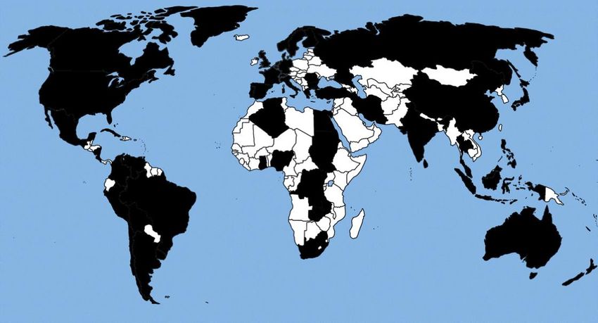
comparison, Eichengreen and Irwin (1995) consider bilateral trade for 34 countries).
Figure 5 summarizes the sample graphically.2 On average, this sample constitutes 82%
of world GDP over this period. Thus, we have a balanced sample of 611 country pairs
over the 20 years from 1920 to 1939, yielding 12,220 observations in total of which 114
are recorded as zeroes.3

 Figure 5: Sample Countries
 Note: 53 sample countries depicted in black

 We code indicator variables for the various blocs discussed by Eichengreen and
Irwin (1995). We consider two trade blocs (the Commonwealth and the Reichsmark
bloc) and two currency blocs (the gold bloc and the sterling area). For countries which
were not in Eichengreen and Irwin’s original sample, we use information on bloc
membership provided by Gowa and Hicks (2013, Table A2). Importantly, these bloc
indicators do not vary over time. In the main, they capture trade flows within blocs
(when both the exporter and the importer are bloc members).

2 The countries in our sample are Algeria, Argentina, Australia, Belgian Congo, Belgium, Bolivia, Brazil,
Bulgaria, Canada, Ceylon, Chile, China, Colombia, Costa Rica, Cuba, Denmark, the Dutch East Indies,
Egypt, Finland, France, Germany, Ghana, Greece, Guyana, Hong Kong, India, Iran, Italy, Japan, Malaysia,
Mexico, the Netherlands, New Zealand, Nicaragua, Nigeria, Norway, Peru, the Philippines, Portugal,
Romania, South Africa, the Soviet Union, Spain, the Sudan, Sweden, Switzerland, Thailand, Turkey, the
United Kingdom, the United States, Uruguay, Venezuela, and Zambia.
3 If we had all possible bilateral pairs over these 20 years, our sample would consist of 55,120 observations

(equal to 53 countries * 52 partners * 20 years). In comparison, Eichengreen and Irwin (1995) cover 561
bilateral pairs for the years 1928, 1935, and 1938 (1683 observations in total). Critically, their data does
not cover the trade collapse of the early 1930s.

 14

Following Eichengreen and Irwin (1995, p. 15), the Commonwealth consists of
seven core countries: Australia, Canada, India, the Irish Free State, New Zealand, South
Africa, and the United Kingdom. We adopt this definition but note that the Irish Free
State is not in our sample. To this, we add the following nine countries: Egypt, Ghana,
Guyana, Hong Kong, Malaysia, Nigeria, Sri Lanka, Sudan, and Zambia. We create two
indicators: a baseline indicator comprising all 15 countries and a narrow indicator
comprising only the first seven countries, all of which were signatories at the Imperial
Economic Conference. The other countries were non-self-governing territories for which
there were some concessions at the Conference, but it is not clear how large these
concessions were. Eichengreen and Irwin (1995, p. 16) define the Reichsmark bloc as
comprising eight countries: Austria, Brazil, Bulgaria, Czechoslovakia, Germany, Greece,
Hungary, and Romania. We adopt this definition but Austria, Czechoslovakia, and
Hungary are not in our sample.
 In terms of gold bloc countries, Eichengreen and Irwin (1995, p. 17) list Belgium,
France, the Netherlands, Poland, and Switzerland. We adopt this definition but note
that Poland is not in our sample. We also add Italy following Gowa and Hicks (2013). As
to the sterling area, Eichengreen and Irwin (1995, p. 17) list the member countries as
Australia, Denmark, Finland, India, the Irish Free State, New Zealand, Norway,
Portugal, South Africa, and Sweden. We adopt this definition with the Irish Free State
again missing. We also add Argentina, Bolivia, Egypt, and Thailand. These 13 countries
(plus the UK) form the core members of the sterling area. In addition, we include the
following seven countries that had reasonably stable exchange rates with respect to
sterling: Ghana, Guyana, Malaysia, Nigeria, Sri Lanka, Sudan, and Zambia.4 Our

4 Our motivation for adding these seven countries comes from a close consideration of their nominal
exchange rates over the sample period. For Ghana, the cedi trades 2 to 1 against sterling throughout the
sample period (the maximum deviation is +/-10%). The Guyanese dollar is initially pegged to sterling at a
rate of 5 to 1. After the British abandonment of the gold standard, there is more variability in the exchange
rate but still in the bounds of +/-10%. For Malaysia, the ringgit trades 8.6 to 1 against sterling throughout
the 1930s with a maximum deviation of +/-10%. For Nigeria, the naira trades 2 to 1 against sterling
throughout the 1930s with a maximum deviation of +/-10%. For Sri Lanka, the rupee trades around 14 to
1 against sterling although there is significant variability in the exchange rate in the early 1920s and the
Great Depression. For Sudan, the Sudanese pound trades at 1 to 1 against sterling with some exchange
rate variability in the early 1920s and the Great Depression. For Zambia, the kwacha/pound trades at 1 to
1 against sterling with some variability in the early 1920s and the Great Depression. Note that we do not
include Hong Kong in this group of countries. The Hong Kong dollar moves from 3.5 units per sterling in
1920 to 16 units in 1939. Visual inspection of the series suggests that there is too much variability

 15

baseline sterling area indicator thus captures 21 countries.5 We also construct a narrow
indicator that only comprises the 14 core members.
 To summarize, within-Commonwealth trade flows represent 8.8% of the
observations in the sample (3.6% based on our narrow definition), and Commonwealth
trade flows with outside partners represent 34% of observations. The within-
Reichsmark bloc only represents a tiny share of our sample—0.3% of observations—and
this bloc’s trade with outside partners represents 17.8% of observations. For trade
within the gold bloc, the fraction of observations is 2.6%, and the corresponding figure
for trade between the gold bloc and outside members is 25.5%. Finally, trade flows
within the sterling area represent 12.9% (8.8% based on our narrow definition) and 43%
with outside members.

3.3 Contours of bilateral trade in the wake of the second great trade
collapse
 As a preliminary exercise, we explore a few interesting contours of the data,
particularly as they relate to the second great trade collapse starting from 1929 and the
trade wars of the 1930s. First, as already documented in Figure 3, real exports fell by
49.1% from 1929 to 1932. However, it remains an open question as to whether this
decline was evenly distributed across country pairs. Figure 6 accordingly plots the
distribution of the percentage declines in the real value of trade between 1929 and 1932
for all bilateral pairs at our disposal. The average change was -43% with a very wide
range of -97% to +374%. However, fully 93% of bilateral pairs suffered a decline in their
trade with one another into 1932. Also, as depicted in Figure 3, a recovery was underway
from 1932 as seen in the flattening of the distribution for the cumulative decline
between 1929 and 1935 and between 1929 and 1938 where the average changes climbed
to -3.2% and +9.7%, respectively. Interestingly though, this recovery was asymmetric as
63% of bilateral pairs were still registering declines in their trade with one another into

(particularly in the mid-1930s possibly related to the strained operation of China’s silver standard) for the
Hong Kong dollar-sterling relationship to be classified as a credible peg.
5 As many countries in the Commonwealth bloc and the sterling area overlap, the correlation between the

two indicators is 0.52. The correlations between the other bloc indicators are close to zero.

 16

1938, suggesting significant changes potentially along the lines of trade and currency
blocs.

 1929-1932
 1929-1935
 1929-1938

 -100% -75% -50% -25% 0% 25% 50% 75% 100%

 Figure 6: Changes in the Value of Bilateral Trade, 1929-1938
 Note: Histogram of percentage changes in trade across country pairs

 Another aspect which we can draw out from the bilateral trade data is the degree
to which commercial policy after 1929 was geared towards reducing bilateral trade
balance deficits and surpluses. Again, this is a claim often asserted in the contemporary
literature (Gordon, 1941; Snyder, 1940), but it has never been documented to the best of
our knowledge. Figure 7 depicts the distribution of the (absolute) value of bilateral trade
balances for the years 1929, 1932, 1935, and 1938, measured in billions of 1990 USD. It
clearly shows a strong progression towards more balanced trade between 1929 (with a
mean imbalance of  = 0.19) and 1932 ( = 0.10), a slight easing between 1932 and 1935
( = 0.12), and a near return to pre-collapse values between 1935 and 1938 ( = 0.15).6
Thus, to the extent that balance of payments pressures were addressed by reducing
bilateral trade deficits, much of this impetus had presumably faded by 1938 when other
considerations had come to the fore.
 A final aspect worth emphasizing here relates to the relatively unappreciated fact
that the second great trade collapse disproportionately affected long-distance country
pairs. As Figure 8 shows, the average trade-weighted distance over the entire period is

6Alternatively, the transition can be seen if we consider the respective ranges rather than averages for
1929 (0.00, 4.75), 1932 (0.00, 2.08), 1935 (0.00, 2.60), and 1939 (0.00, 4.22).

 17

5,675 km. However, while the average trade-weighted distance remains relatively stable
until 1929, there is a substantial and sudden drop to 5,108 km in 1931. This measure
then starts to rise, reaching a peak of 6,013 km in 1937.

 1929
 1932
 1935
 1938

 0.00 0.05 0.10 0.15 0.20 0.25 0.30

 Figure 7: Bilateral Trade Balances (absolute values), 1929-1938
 Note: Histogram of trade balances across country pairs in billions of 1990 USD

 6050

 5850

 5650

 5450

 5250

 5050
 1920 1921 1922 1923 1924 1925 1926 1927 1928 1929 1930 1931 1932 1933 1934 1935 1936 1937 1938 1939

 Trade-weighted distance by year Average weighted distance, 1920-1939

 Figure 8: Trade-Weighted Distances, 1920-1939
 Note: Weighted average of bilateral distances in km across country pairs

 18

These patterns of stability, sharp decline, and substantial recovery can be roughly
discerned across all countries and within and outside all trade and currency blocs with
two notable exceptions. First, within the Commonwealth the average trade-weighted
distance exhibits an upward secular trend throughout the 1920s and 1930s. What is
more, there was no decline in this measure—indeed, there was an increase—during the
second great trade collapse, suggesting that trade between Commonwealth countries
was disrupted proportionally less.7 Second, within the sterling area the average trade-
weighted distance exhibits a slight but steady decline throughout the 1920s and 1930s.
 Finally, all these aspects suggest that in some measure, the effects of the trade
wars of the early 1930s were of relatively short duration. Bilateral trade volumes and
bilateral trade balances were rising on average from their lows in the early 1930s while
trade-weighted distances had recovered by 1935. However, the possibility remains that
the trade wars of the early 1930s mainly served to intensify pre-existing efforts towards
the formation of trade blocs which dated from—and presumably, even before—1920.

3.4 Gravity regressions
 We run panel gravity regressions based on our annual bilateral trade flows over
the period from 1920 to 1939. All regressions include time-varying exporter and
importer fixed effects using OLS. We are particularly interested in the behavior of the
distance elasticity and indicator variables for the four blocs under consideration.8 A
standard gravity regression with logarithmic distance as the only regressor of interest
yields a distance elasticity of -0.69 with a standard error of 0.02. The R-squared stands
at 72%. This basic finding confirms the well-known result that gravity is indeed
applicable for the pre-1950 world (see Jacks, Meissner, and Novy, 2011).
 In the next step, we add indicator variables for the four blocs and allow them to
vary over time. These regressions are similar in spirit to those reported by Eichengreen
and Irwin (1995, Table 2) and Gowa and Hicks (2013, Table 3). The main difference is
that we use data for every consecutive year over this period. This allows us to see time

7The same observation holds for our narrow Commonwealth dummy that captures fewer countries.
8For the results reported here, we do not include an indicator for a common border between two
countries as it does not display any systematic pattern over time, and it is often insignificant.

 19

trends more clearly.9 We present the results in Figure 9 where we depict the value of the
coefficients in every year for our four blocs: within the Commonwealth, within the
Reichsmark bloc, within the gold bloc, and within the sterling area. To achieve
comparability, we normalize these coefficients to 100 for the year 1920. The gold bloc
and sterling area coefficients exhibit no particular trend over time. The Reichsmark bloc
coefficient initially falls but then strongly rises after 1932. However, the most striking
observation is the rise of within-Commonwealth trade. The Commonwealth coefficient
more than doubles throughout the interwar period, reaching a value of 269 in 1939. It
shows a particularly strong upward trend after 1931, suggesting an intensification of
trade within the Commonwealth due to the imposition of discriminatory trade policies
by Britain (de Bromhead et al., 2019a).10

 300

 250

 200

 150

 100

 50

 0
 1920 1921 1922 1923 1924 1925 1926 1927 1928 1929 1930 1931 1932 1933 1934 1935 1936 1937 1938 1939

 Commonwealth RM bloc Gold bloc Sterling area

 Figure 9: Bilateral Trade within Blocs, 1920-1939
 Note: Coefficients for bloc membership by year, normalized to 1920 = 100

9 Since we use exporter and importer fixed effects, we cannot simultaneously include both intra-bloc and
extra-bloc indicators due to collinearity. This is in direct contrast with Eichengreen and Irwin (1995) who
do not employ importer and importer fixed effects and thus do not control for multilateral resistance
effects. Note that since the bloc indicators do not vary over time, we do not add pair fixed effects.
10 Formally, we cannot reject the joint equality of the Commonwealth coefficients (p-value = 0.29) since

confidence intervals are quite large. Results are very similar when we use the narrow definitions of the
Commonwealth and the sterling area.

 20

In Figure 10, we plot distance elasticities for each bloc that are allowed to vary
over time. That is, we allow for a triple interaction of distance by time by bloc.11 Again,
we normalize these coefficients to 100 for the year 1920. This converts negative
coefficients on distance into positive shares of the original effect. Thus, the distance
elasticity for the Commonwealth stands at -1.19 in 1920 (index value = 100.0) and -0.31
in 1929 (index value = 26.2). What is most remarkable from this figure is the fact that
the distance elasticity for the Commonwealth: (1) is consistently falling throughout the
1920s and 1930s12 and (2) attains a value of zero in 1939.13

 225

 200

 175

 150

 125

 100

 75

 50

 25

 0
 1920 1921 1922 1923 1924 1925 1926 1927 1928 1929 1930 1931 1932 1933 1934 1935 1936 1937 1938 1939

 Commonwealth RM bloc Gold bloc Sterling area

 Figure 10: Bilateral Distance Elasticities within Blocs, 1920-1939
 Note: Value of regression coefficient for distance by year, normalized to 1920 = 100

 Naturally, this result is linked to the steady rise in the average trade-weighted
distance of bilateral trade within the Commonwealth documented in section 3.3: the
longer the distance covered by the average trade flow, the less sensitive trade appears to
be to distance in the context of regression analysis. Figure 10 also reveals roughly
constant distance elasticities for the gold and Reichsmark blocs, while there appears to

11 We also estimate distance elasticities for the omitted group of pairs that are captured by neither the
Commonwealth, the Reichsmark bloc, the gold bloc, nor the sterling area. This group of “other” pairs has
a distance elasticity of around -0.30 and is fairly stable over time.
12 Eichengreen and Irwin (1995) stress a similar result for the singular year of 1928, citing early evidence

by Schlote (1952) and Thorbecke (1960) who “are skeptical that imperial preference was primarily
responsible for the growth of intra-Commonwealth trade [as] the trend was evident earlier…”
13 At the same time, we cannot reject the joint equality of the annual Commonwealth distance elasticities

(p = 0.24).

 21

be a modest—albeit insignificant—increase in the trade-diminishing effects of distance
for the sterling area.
 In summary, we conclude that interwar trade patterns can be roughly
characterized by two dominant observations. First, there was a persistent long-run trend
towards the “death of distance” in the context of bilateral trade flows within the
Commonwealth, but decidedly nowhere else. Second, there were also substantial
increases in bilateral trade flows associated with both the Commonwealth and the
Reichsmark bloc from 1931 and 1932, respectively. However, in the case of the
Commonwealth, the second great trade collapse and its related trade wars seemed to
only reinforce a pre-existing trend built around a surging trade bloc, spanning nearly all
continents of the globe.14

3.5 Variance decomposition
 As an alternative to regression coefficients, we now consider variance
decompositions. As before, we focus on distance elasticities and indicator variables for
the four blocs. While we have shown above that both show systematic patterns in
regressions, so far we have not ascertained their relative importance in explaining trade
patterns. A decomposition of the variance of trade flows is well-suited for that purpose.
 We follow the variance decomposition approach suggested by Fields (2003).
Although his focus is on income inequality in the labor market, the methodology can be
applied more generally to linear specifications such as the gravity equation in
logarithmic form. The objective is to explain the variance of the dependent variable
which for us is the logarithm of bilateral trade flows. The approach used by Fields
(2003) determines the share of the variance of the dependent variable which can be
attributed to each individual regressor on the right-hand side. Specifically, the variance
share attributed to an individual regressor is given as
 ( ,ln )
 (2) = ,
 (ln )

14Kindleberger (1989, p. 161) explains that the British orientation towards the Commonwealth/Empire to
some extent had its origins in World War I. Referring to the duties imposed by the UK in the 1915
McKenna budget, he writes: “The tariffs, moreover, made it possible for the United Kingdom to
discriminate in trade in favour of the British Empire, something it could not do under the regime of free
trade which had prevailed since the 1850s.”

 22

where m is the regression coefficient of the dependent variable ln x (logarithmic
bilateral trade) on the explanatory variable zm (logarithmic distance or a bloc indicator),
holding all other explanatory variables constant. Cov and Var denote the covariance and
variance, respectively.
 We apply this methodology to the annual gravity regressions with exporter and
importer fixed effects, revealing that bilateral distance is the most important
determinant for explaining the variance of bilateral trade with a contribution of 7.4% on
average.15 But as the top line in Figure 11 illustrates, the contribution of distance
declines from almost 9% in the early 1920s to just over 6% by the late 1930s. Again, this
trend predates the second great trade collapse, suggesting that distance becomes less
influential as a determinant of trade flows over the 1920s and 1930s.

 0.10

 0.09

 0.08

 0.07

 0.06

 0.05

 0.04

 0.03

 0.02

 0.01

 0.00
 1920 1921 1922 1923 1924 1925 1926 1927 1928 1929 1930 1931 1932 1933 1934 1935 1936 1937 1938 1939

 Commonwealth RM bloc Sterling area Distance

 Figure 11: Variance Decomposition for Bilateral Trade Flows, 1920-1939
 Note: Share of variation in bilateral trade explained by independent variables

 Turning to the indicator variables for the four blocs, we find that they are not
nearly as important in explaining the variance of bilateral trade since individual bloc
contributions never exceed 2%. In terms of the individual bloc contributions, the
Commonwealth dummy explains around 1% of the variance on average. However, this
contribution increases over time especially after 1931. This finding is consistent with our

15This contribution of distance is in line with results for geographic indicators and transport cost variables
in a study by Chen and Novy (2011) who explain the variance of trade costs. It is also roughly in the same
ballpark as contributions of key regressors such as experience and schooling in the Mincer regressions
decomposed by Fields (2003).

 23

earlier regression results. The contributions of the gold and Reichsmark blocs are
negligible.16 The contribution of the sterling area averages a relatively healthy 1.1% but
with a slight decline over time. In general, this result means that geography in the form
of bilateral distance is clearly the dominant determinant of bilateral trade, while
political institutions in the form of trade and currency blocs are of second order. We
were not able to obtain this insight from standard gravity coefficients alone.
 What explains the remaining variance? Most of the variance is explained by the
residuals (88% on average). This is hardly surprising since the residuals absorb all the
variance in the data that cannot be explained by the gravity model. This finding is
typical (for instance, see Table 3 in Fields, 2003). Although exporter and importer fixed
effects are important theoretically as they represent income and multilateral resistance
variables, they are not pair-specific and therefore not crucial for explaining bilateral
flows. In our sample, exporter and importer fixed effects combined explain 3.2% of the
variance on average. This share has no trend over time, but it does dip below 2% in
1932-1933, suggesting that country-specific factors were less important during the
depths of the second great trade collapse.

4. The lessons and limits of historical parallels
 To summarize, we have argued that the trade wars of the early 1930s were
executed primarily against all trade partners and in a distinctly uncoordinated fashion
with instances of bilateral retaliation being minor and rare in comparison. Instead, the
overwhelming aim of both tariff and non-tariff barriers was as a defense to the
deflationary forces embedded in the global economy at the time. Moreover, using an
extensive panel of annual bilateral trade data for the entirety of the interwar period, we
have found that the effects of the trade wars of the early 1930s were of relatively short
duration and that they mainly served to intensify pre-existing efforts towards the
formation of trade blocs, above all the British Commonwealth.

16The respective contributions are 0.1% and -0.6% on average. The negative sign of the gold bloc
contribution is due to the negative coefficient on the gold bloc indicator in the underlying regressions.
That is, relative to the omitted group (all country pairs that do not belong to other blocs), gold bloc pairs
trade less on average after we control for bilateral distance and exporter and importer fixed effects.
Formally, a negative contribution in the decomposition is only possible if the regression coefficient carries
the opposite sign of the covariance between the regressor and the dependent variable.

 24

By way of conclusion, we offer up some observations, highlighting the lessons and
limits of historical parallels as they relate to the notion of trade wars. First, the present
day does seem to share some common features with the 1930s. In particular, there is the
prospect that a formerly dominant multilateral trading system is in danger of being
replaced by a set of bilateral “deals”. Thus, the 1930s witnessed the unraveling of an
informal, but long-standing agreement among most nations of the world in which
commercial relations were guided by the distinctly multilateral principles laid out in the
Cobden-Chevalier treaty of 1860. But during the better part of 20 years it took to
rediscover and institutionalize these features in the form of the GATT, many of these
same nations first scrambled to erect protectionist walls against all comers and then to
punch holes through them via bilaterally-negotiated systems of preferences.
 At the moment, we have not witnessed a wholesale collapse of the modern
trading system. This is partially for the fact that policymakers seem to have learned
some of the lessons of interwar history by not responding in a general fashion to
unilateral moves toward protectionism. This does, however, raise the prospect that the
trade wars of the present day may serve the same purpose of those in the 1930s, that is,
the intensification of existing and nascent trade blocs. Thus, it requires no great
imagination to see a future in which consumers’ preferences, firms’ perceptions of
uncertainty, and states’ apprehensions of one another endogenously lead to a
reorientation of world trade around China- and US-centric trade blocs.
 Of course, one particularly telling difference of the present day from the interwar
period comes from the composition of trade. Even a brief review of the historical
literature on interwar trade reveals that this was still a world dominated by inter-
industry trade with only 43% of world exports being classified as manufactured goods
(Jacks and Tang, 2018). In contrast, manufactured goods now constitute the
overwhelming majority of world exports, and the subsequent fragmentation of
production has given rise to both a heightened sensitivity of trade flows to protectionist
measures and a heightened sense of mutual interdependence across countries (Baldwin,
2016; Feenstra, 1998). Thus, the extent to which global value chains can be unraveled
arguably places limits on how far this prospective bloc-based trajectory for world trade
might proceed.

 25

References
Anderson, J.E. and E. van Wincoop (2003), “Gravity with Gravitas: A Solution to the
 Border Puzzle.” American Economic Review 93(1): 170-192.
Baldwin, R. (2016), The Great Convergence: Information Technology and the New
 Globalization. Boston: Harvard University Press.
Berglund, A. (1935), “The Reciprocal Trade Agreements Act of 1934.” American
 Economic Review 25(3), 411-425.
de Bromhead, A., A. Fernihough, M. Lampe, and K.H. O’Rourke (2019a), “When Britain
 Turned Inward: The Impact of Interwar British Protection.” American Economic
 Review 109(2), 325-352.
de Bromhead, A., A. Fernihough, M. Lampe, and K.H. O’Rourke (2019b), “The Anatomy
 of a Trade Collapse: The UK, 1929-33.” European Review of Economic History
 23(2), 123-144.
Capie, F. (1983), Depression and Protectionism: Britain between the Wars. London:
 George Allen and Unwin Limited.
Chen, N. and D. Novy (2011), “Gravity, Trade Integration, and Heterogeneity across
 Industries.” Journal of International Economics 85(2), 206-221.
Eichengreen, B. (1992), Golden Fetters: The Gold Standard and the Great Depression,
 1919-1939. New York: Oxford University Press.
Eichengreen, B. and D.A. Irwin (1995), “Trade Blocs, Currency Blocs and the
 Reorientation of World Trade in the 1930s.” Journal of International Economics
 38(1), 1-24.
Eichengreen, B. and D.A. Irwin (2010), “The Slide to Protectionism in the Great
 Depression: Who Succumbed and Why?” Journal of Economic History 70(4),
 871-891.
Eichengreen, B. and P. Temin (2000), “The Gold Standard and the Great Depression.”
 Contemporary European History 9(2), 183-207.
Estevadeordal, A., B. Frantz, and A.M. Taylor (2003), “The Rise and Fall of World
 Trade, 1870-1939.” Quarterly Journal of Economics 118(2), 359–407.
Feenstra, R.C. (1998), “Integration of Trade and Disintegration of Production in the
 Global Economy.” Journal of Economic Perspectives 12(4), 31-50.
Fields, G.S. (2003), “Accounting for Income Inequality and Its Change: A New Method,
 with Application to the Distribution of Earnings in the United States.” Research
 in Labor Economics 22, 1-38.
Findlay, R. and K.H. O’Rourke (2008), Power and Plenty: Trade, War, and the World
 Economy in the Second Millennium. Princeton: Princeton University Press.
Friedman, M. and A.J. Schwartz (1963), A Monetary History of the United States, 1867-
 1960. Princeton: Princeton University Press.
Gordon, M.S. (1941), Barriers to World Trade: A Study of Recent Commercial Policy.
 New York: The Macmillan Company.
Gowa, J. and R. Hicks (2013), “Politics, Institutions, and Trade: Lessons of the Interwar
 Era.” International Organization 67(3), 439-467.
Grossman, G.M. (1998), Comment. In J. Frankel (Ed.), The Regionalization of the
 World Economy. Chicago: University of Chicago Press.
Hart, M. (2002). A Trading Nation: Canadian Trade Policy from Colonialism to
 Globalization. Vancouver: University of British Columbia Press.

 26