Circuit encapsulation for efficient quantum computing based on controlled many-body dynamics
←
→
Page content transcription
If your browser does not render page correctly, please read the page content below
Circuit encapsulation for efficient quantum computing based on controlled many-body dynamics
                                                                                 Ying Lu,1 Peng-Fei Zhou,1 Shao-Ming Fei,2, 3, ∗ and Shi-Ju Ran1, †
                                                                                 1
                                                                                   Department of Physics, Capital Normal University, Beijing 100048, China
                                                                         2
                                                                             School of Mathematical Sciences, Capital Normal University, Beijing 100048, China
                                                                              3
                                                                                Max-Planck-Institute for Mathematics in the Sciences, 04103, Leipzig, Germany
                                                                                                          (Dated: March 30, 2022)
                                                                Controlling the time evolution of interacting spin systems is an important approach of implementing quantum
                                                             computing. Different from the approaches by compiling the circuits into the product of multiple elementary
                                                             gates, we here propose the quantum circuit encapsulation (QCE), where we encapsulate the circuits into different
                                                             parts, and optimize the magnetic fields to realize the unitary transformation of each part by the time evolution.
                                                             The QCE is demonstrated to possess well-controlled error and time cost, which avoids the error accumulations
                                                             by aiming at finding the shortest path directly to the target unitary. We test four different encapsulation ways to
                                                             realize the multi-qubit quantum Fourier transformations by controlling the time evolution of the quantum Ising
                                                             chain. The scaling behaviors of the time costs and errors against the number of two-qubit controlled gates are
                                                             demonstrated. The QCE provides an alternative compiling scheme that translates the circuits into a physically-
                                                             executable form based on the quantum many-body dynamics, where the key issue becomes the encapsulation
                                                             way to balance between the efficiency and flexibility.
arXiv:2203.15574v1 [quant-ph] 29 Mar 2022

                                                                    I.   INTRODUCTION                                    plement the measurement-based quantum computation [34–
                                                                                                                         40]. However, the utilizations of the many-body dynamics
                                               Quantum computing is recognized as a promising scheme                     for quantum computing [25, 28, 29] are much less explored,
                                            being superior to the classical computing for its exponential                where more valid schemes are desired.
                                            speed-up by executing multiple computational tasks parallelly                   For all known quantum computing platforms, severe chal-
                                            in different quantum channels [1–3]. With the fast growth                    lenges are caused by the inevitable noises. The noises might
                                            of the number of controllable qubits, efficient compiling of                 induce computational errors, making the results unstable or
                                            the quantum algorithms to the physically-executable forms                    unreliable. One way of fighting against the errors is to add the
                                            becomes increasingly important. A mainstream compiling                       error correction codes [41], such as Toric codes [42], which
                                            scheme is to transform the circuit into the product of exe-                  will further increase the complexity of the circuits. Noises
                                            cutable elementary gates, which are the quantum version of                   will also lead to decoherence, meaning that the qubits will
                                            the instruction set [4–8]. The instruction set should be con-                gradually become less entangled and lose the superiority over
                                            structed according to the physical mechanism of the hardware.                the classical computing. Prolonging the coherence time and
                                            For instance, a quantum computer formed by the supercon-                     reducing the time cost so that the quantum computing is ex-
                                            ducting circuits can use the QuMIS [9] as the instructive set.               ecuted within the coherence duration belong to the signifi-
                                            For the quantum photonic circuits, the elementary gates repre-               cant and challenging issues for quantum computing (see, e.g.,
                                            sent certain basic operations on single photons [10, 11]. The                Refs. [43–46]).
                                            efficiency of compiling a given quantum algorithm with a cho-                   Concerning the quantum computing based on the controlled
                                            sen instruction set can be characterized by the depth of the                 many-body dynamics, we here propose the quantum circuit
                                            compiled circuit.                                                            encapsulation (QCE) to optimize the magnetic fields for effi-
                                               Another important approach of quantum computing is by                     cient implementation of quantum circuits. Considering a tar-
                                            controlling the dynamics of quantum systems. A representa-                   get unitary (dubbed as quantum capsule, Q-cap in short) that
                                            tive platform is the nuclear magnetic resonance system, where                might be formed by one or multiple gates, the idea is to op-
                                            quantum gates or algorithms [12–15], such as the quantum                     timize the magnetic fields so that the time-evolution operator
                                            factoring [16] and search [17–19] algorithms, have been real-                realizes the unitary. In the QCE, a quantum circuit can be con-
                                            ized by the radio-frequency pulse sequences. The efficiency                  sidered as one Q-cap or divided into multiple Q-caps, corre-
                                            can be characterized by the time cost for the controlling. For               sponding to different encapsulation ways. As the intermediate
                                            the two-qubit gates, such as the controlled-not (CNOT) gate,                 processes given by the gates within a Q-cap will not appear in
                                            the time costs with optimal control have theoretically given                 the time evolution, different encapsulation ways result in dif-
                                            bounds [20–22]. For the N -qubit gates with N > 2, such                      ferent flexibilities. A key issue in the QCE is thus the balance
                                            bounds are not rigorously given in most cases, and variational               between the efficiency and flexibility.
                                            methods including the machine learning (ML) techniques are                      We compare four different ways of encapsulation for the
                                            used in the optimal-control problems [23–33]. Besides, the                   realization of the N -qubit quantum Fourier transformation
                                            quantum many-body systems have also been used to im-                         (QFT) [47–49], and demonstrate the scaling behaviors of the
                                                                                                                         errors and time costs against the number of controlled gates.
                                                                                                                         Specifically, we show a slow linear growth of the time cost
                                                                                                                         with well-controlled errors ε ∼ O(10−1 ) up to N = 6, by
                                            ∗   Corresponding author. Email: feishm@cnu.edu.cn                           considering the whole circuit as one Q-cap. For lager N ’s, the
                                            †   Corresponding author. Email: sjran@cnu.edu.cn                            block-wise encapsulation is speculated to be a proper choice,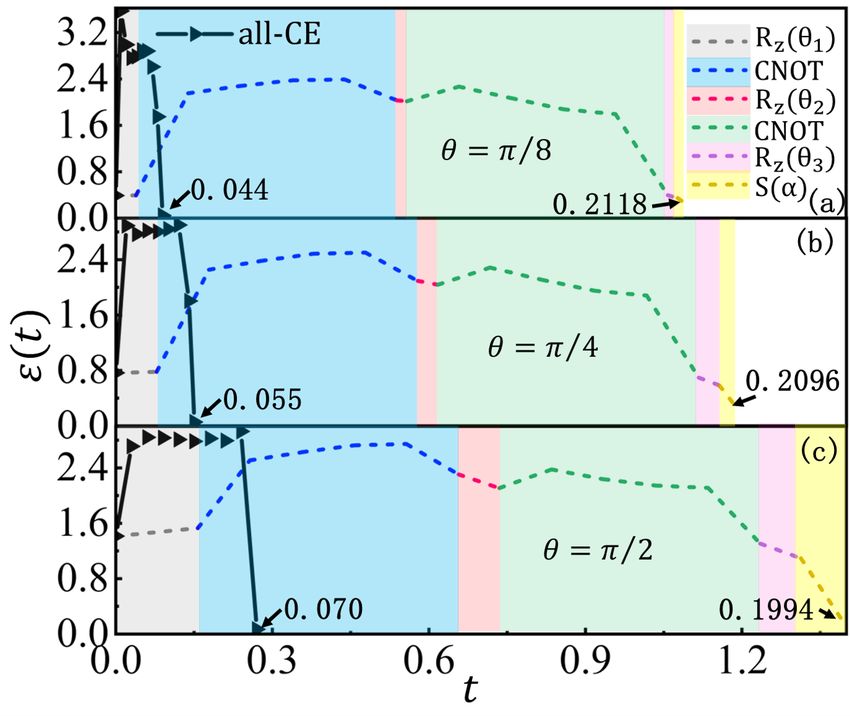
2

where we expect moderate linear growths of the time costs                      k = 1, · · · , K and K = Tτ ). In other words, the magnetic
and errors.                                                                    fields are allowed to change for K times. The magnetic fields
                                                                               are updated as

        II.    QUANTUM CIRCUIT ENCAPSULATION                                                                                    ∂ε
                                                                                                   hα      α
                                                                                                    n,k ← hn,k − η                   ,              (6)
                                                                                                                               ∂hα
                                                                                                                                 n,k
  Consider a quantum circuit Û that consists of M gates
                                        QM                                     where the gradients ∂h∂ε     are obtained by the automatic dif-
{Ĝ[m] } (m = 1, · · · , M ) with Û = m=1 Ĝ[m] . We here                                              α
                                                                                                        n,k

propose to find the time-dependent Hamiltonian Ĥ(t), and its                  ferentiation in Pytorch [52]. We use the optimizer Adam [53]
evolution operator for the time duration T optimally gives the                 to dynamically control the learning rate η.
                                                                                  We employ two algorithms to implement the optimizations,
unitary transformation of the target circuit Û , i.e.,
                                                                               namely the global time optimization (GTO) and fine-grained
                                             RT
                             Û ' e−i         0
                                                  Ĥ(t)dt
                                                            .            (1)   time optimization (FGTO) [32]. GTO is a simple gradient-
                                                                               descent method, where the strengths of the magnetic fields
We take the Plank constant ~ = 1 for simplicity.                               for all time slices are updated simultaneously by Eq. (6). For
   We constrain that the adjustable parameters of the Hamil-                   the simple cases such as the two-qubit unitaries, GTO shows
tonian only concerns the one-body terms, i.e., the magnetic                    high accuracy. However, for more complicated cases such as
fields. Specifically, we take the quantum Ising model as an                    the N -qubit QFT with a large N , GTO could be trapped in
example, where the Hamiltonian reads                                           a local minimum. The FGTO is thus employed, where the
             X                      X                                          key idea is to asymptotically fine-grain the time discretization
     Ĥ(t) =     Jnn0 Ŝnz Ŝnz 0 −  [hxn (t)Ŝnx + hyn (t)Ŝny ], (2)         (characterized by τ ) to avoid the possible local minimums.
                   nn0                            n                            See more details in Ref. [32].
                                                                                  The way of encapsulation is flexible. In general, we con-
with Ŝnα the spin operator in the α direction (α = x, y, z),
                                                                               sider to separate the gates in the circuit into P groups as
Jnn0 the coupling strength between the n-th and n0 -th spins,
and hαn (t) the magnetic field along the α direction on the n-th                                  P                               Mp
spin at the time t. We assume Jnn0 to be constant and hα
                                                                                                  Y                               Y
                                                              n (t)                        Û =         Ĝ [p] , with Ĝ [p] =          Ĝ[mj ] .   (7)
to be adjustable with time.                                                                       p=1                             j=1
   The goal becomes optimizing the magnetic fields to mini-
mize the difference between the time-evolution operator and                    The unitary Ĝ [p] consists of Mp gates from the target cir-
the target unitary Û . To this end, a simplest choice is to mini-             cuit and is named as a quantum capsule (Q-cap). We have
                                                                               PP
mize the following loss function defined as                                        p=1 Mp = M . We optimize the magnetic fields indepen-
                                                  RT                           dently for each Q-cap, where we define the loss function for
                          ε = Û − e−i            0
                                                       Ĥ(t)dt
                                                                 .       (3)   Ĝ [p] as
                                                                                                                        R Tp
The magnetic fields are optimized using the gradient descent                                                       −i            Ĥ(t)dt
                                                                                              εp = Ĝ [p] − e            Tp−1
                                                                                                                                           ,        (8)
as
                                                          ∂ε                   wth ∆Tp = Tp − Tp−1 the evolution duration for realizing
                         hα        α
                          n (t) ← hn (t) − η                    ,        (4)
                                                        ∂hα
                                                          n (t)                Ĝ [p] and the total time T = TP . The magnetic fields during
with η the gradient step or learning rate. Since such an op-                   Tp−1 ≤ t < Tp are optmized by minimizing εp .
timization cares about the distance between the unitary given                      As a natural encapsulation way, the main advantage of the
by the whole circuit and the evolution operator at the final                   all-CE (meaning to treat the whole circuit as one Q-cap) is
time T , the evolution at t < T will not give any intermediate                 straightforward, which is to reduce the time cost and error by
results from the gates within the circuit. We dub such a circuit               directly finding the path to the final unitary. One may com-
encapsulation (CE) way as all-CE.                                              pare, for instance, with a naive way by considering each gate
   In the numerical simulation, we take the Trotter-Suzuki                     in the circuit as a Q-cap (naive-CE). First, the errors of se-
form [50, 51] and discretize the total time T to K̃ identical                  quentially realizing each gate would in general accumulate.
slices. The evolution operator can be approximated as                          We expect much less errors by directly minimizing the differ-
                                                                               ence between the target and the final evolution operator in the
          Û (T ) = e−iτ Ĥ(K̃ τ̃ ) . . . e−iτ̃ Ĥ(2τ̃ ) e−iτ̃ Ĥ(τ̃ )         all-CE, which is similar to the end-to-end optimization strat-
                           1
                           Y                                                   egy widely used in the field of ML and ML-assisted physical
                     =            e−iτ̃ Ĥ(k̃τ̃ ) .                      (5)   approaches (see, e.g., Ref. [27]).
                          k̃=K̃
                                                                                   Second, a unitary can be compiled into different circuits
                                                                               by applying different quantum instruction sets. One may use
              T
with τ̃ =     that controls the Trotter-Suzuki error. For vary-
              K̃
                                                                               the depth of the circuit to characterize the efficiency of the
ing the magnetic fields, we introduce τ = κτ̃ with κ a pos-                    compilation. The depth would usually change if one turns
itive integer, and assume hα  n (t) to take the constant value                 to a different instruction set. From the perspective of QCE,
hα          α
  n (t) = hn,k during the time of (k − 1)τ ≤ t < kτ (with                      the efficiency should be characterized by the total time cost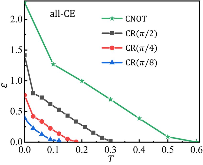
3
with θ the factor of phase shift. A normal treatment is to de-
compose a CR into the product of single-qubit rotations R̂z
and CNOT Ĉ as
CR(θ) = Ŝ(α)R̂z (θ1 )Ĉ R̂z (θ2 )Ĉ R̂z (θ3 ), (11)
satisfying R̂z (θ1 )R̂z (θ2 )R̂z (θ3 ) = I [57] and Ŝ(α) = eiα a
phase factor.
Taking θ = π8 , π4 , and π2 , Fig. 2 compares the error [ε in
Eq. (3)] by encapsulating the CR(θ) (all-CE) and that by en-
capsulating gate by gate after decomposing it into the elemen-
tary gates [Eq. (11)] (named as the decomposed CE, decomp-
CE in short). Since only the two-qubit gates are involved, we
choose GTO to optimize the magnetic fields. The dashed lines
(decomp-CE) and solid lines with triangles (all-CE) show the
0 0
Rt
time-dependent error ε(t) = Û − e−i 0 Ĥ(t )dt . Note in all
cases, the magnetic fields are always optimized according to
the definitions of the Q-caps. The time costs of realizing dif-
ferent elementary gates in the decomp-CE are illustrated by
FIG. 1. (Color online) The time-dependent error ε(t) =
−i 0t Ĥ(t0 )dt0
R the colored shadows. The time cost of the all-CE is indicated
Û − e versus the time t. The dashed lines and the by the x-coordinate of the last triangle, which is about five
solid lines with triangles show the ε(t) by the decomp-CE and all- times shorter than the decomp-CE. For a single-qubit rotation
CE, respectively. The colored shadows indicate the time costs for R̂α (θ), it can be written as the one-body evolution operator
realizing the the gates in the right-hand-side of Eq. (11) (decomp-
with the magnetic field along the corresponding direction, i.e.,
CE).
α α
Ŝ α
R̂α (θ) = e−iθŜ ⇔ Û (hα , T ) = e−iT h . (12)
for reaching the preset error. An obvious drawback of all-
Therefore, the time cost of R̂α (θ) is estimated as T = hθα .
CE is that one cannot extract the relevant information of the
Without losing generality, we here take hα = 10 to estimate
intermediate process from the gates within the circuit (i.e., Q-
the time costs of the single-qubit rotations.
cap). Therefore, a proper encapsulation should balance be-
An important observation is that even the time cost of a
tween the efficiency and the ability of extracting the inter-
single CNOT is larger than that of the CR(θ) by the all-CE.
mediate information, according to the specific computational
The all-CE of CR(θ) also leads to much lower errors with
tasks or purposes. For example, the frequently-use circuits,
ε ∼ O(10−2 ). For the decomp-CE, the error accumulates and
such as the QFT applied in many quantum algorithms includ-
finally reaches O(10−1 ) that is about ten times larger than
ing Shor’s [54] and Grover search [55] algorithms, can be en-
that by the all-CE. Therefore, from the perspective of QCE, it
capsulated into Q-caps for the convenience of the future use.
is not a wise choice to decompose the CR(θ) into the product
of CNOT and the single-qubit rotations.
Fig. 2 shows how the error ε varies with the total evolution
III. RESULTS OF QUANTUM CIRCUIT ENCAPSULATION
duration T for realizing the CNOT and CR(θ) by the all-CE. In
all cases, ε decreases with T as expected, meaning that higher
Below, we take Hamiltonian for the time evolution as the accuracy can be reached by increasing the evolution time. Be-
nearest-neighbor Ising chain, where the coupling constants low, the time cost of a Q-cap is determined by the T when the
satisfy ε reaches about 10−1 . Again, we show that CR(θ) requires
much shorter time than CNOT to obtain a similar accuracy.
2π for n0 = n + 1
Jnn =
0 . (9) For the CR(θ), the time cost increases with θ for all T ’s.
0 otherwise
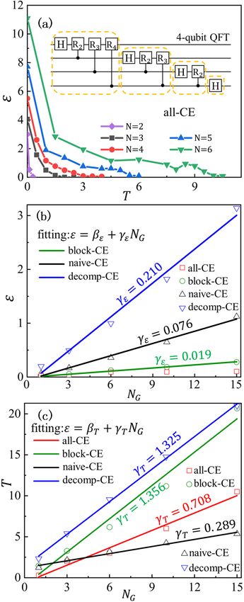
Fig. 3(a) demonstrates the error ε [Eq. (3)] of realizing the
We set the magnetic fields along the spin-z direction as zero, N -qubit QFT by all-CE with different total time duration T ,
and allow to adjust the fields only along the spin-x and y di- for N = 2, · · · , 6. The inset illustrates the circuit with N = 4
rections. Such a restriction often appears in the controlling by as an example. In general, one can obtain lower ε by increas-
the radio-frequency pulses [56]. ing T . Longer evolution time is required to reach a preset
As a simple example, we consider the two-qubit controlled- error if N increases.
R (CR) gate that satisfies We further compare the errors (ε) and the corresponding
time costs (T ) using different encapsulation ways. The block-
1 0 0 0 CE of the QFT circuit is illustrated by the dashed hollow
0 1 0 0 squares in the inset of Fig. 3(a). The circuit is divided into sev-
CR(θ) = (10)
0 0 1 0 eral blocks according to the positions of the Hadamard gates
iθ H. Each block is treated as a Q-cap for optimizing the mag-
0 0 0 e4
FIG. 2. (Color online) The error ε [Eq. (3)] with different total evolu-
tion duration T for the CNOT and CR(θ) (with θ = π/2, π/4, π/8)
by the all-CE.
netic fields. The block-CE possesses certain flexibility. For in-
stance, the last (Ñ + 1) blocks form the circuit of the Ñ -qubit
QFT. We also try the naive-CE, where we treat each gate in the
QFT circuit as a Q-cap for the optimization of the magnetic
fields. For the decomp-CE, we decompose each CR gate to
the product of the CNOT and single-qubit rotations following
Eq. (11), and then treat each gate as a Q-cap for optimization.
There is an important detail we shall stress. For the N -qubit
QFT, if a Q-cap only concerns N 0 qubits with N 0 < N , we
use the quantum Ising model of just the N 0 qubits to imple-
ment the time evolution. It means that the irrelevant couplings
outside such a N 0 -qubit quantum Ising model are turned off.
Surely we can keep all the couplings in the N -qubit system
and find the optimal magnetic fields to realize the unitary act-
ing on the N 0 -qubit subsystem. This, however, will lead to
much lower accuracies than those by turning off the irrele-
vant couplings. We therefore choose to turn off the irrelevant
couplings in the block-CE, naive-CE, and decomp-CE, as the
baselines compared with the all-CE.
Fig. 3(b) shows how the error ε of realizing the QFT in-
creases with the number of the CR gates NG using different
encapsulation ways. As we require εp ' 10−1 [Eq. (8)] for
the optimization of each Q-cap, we have ε ' 10−1 for the all-
CE as there is only one Q-cap [red squares in Fig. 3(b)]. For
other encapsulation ways, there exist multiple Q-caps, where
the errors accumulate. Consequently, we observe that ε in-
creases linearly with NG as
ε = γε NG + βε , (13) FIG. 3. (Color online) (a) The error ε [Eq. (3)] with different total
evolution duration T for the N -qubit QFT with N = 2, · · · , 6 by the
with the slope γε ' 0.019, 0.076, and 0.210 for the block-CE, all-CE. The inset illustrates the circuit of the 4-qubit QFT. In (b) and
naive-CE, and decomp-CE, respectively. We have the coeffi- (c), we show the errors ε and time costs T using the all-CE, block-
cient of the determinant that characterizes the error of a linear CE, naive-CE, and decomp-CE against the number of CR gates NG .
fitting as R2 ' 0.991, 0.989, and 0.988, respectively. The errors from the all-CE are controlled to be about 10−1 . The solid
The corresponding time costs T for reaching the errors in lines in (b) show the linear fittings of ε for the block-CE, naive-CE,
Fig. 3(b) are given in Fig. 3(c). The linear dependence of T on and decomp-CE, with the coefficient of determinant R2 ' 0.991,
NG is observed for all four kinds of encapsulation ways with 0.989, and 0.988, respectively. The solid lines in (c) show the linear
fittings of T for the all-CE, block-CE, naive-CE, and decomp-CE
T = γT NG + βT . (14) with R2 ' 0.982, 0.975, 0.984, and 0.999, respectively.5
The naive-CE gives the smallest slope with γT ' 0.289 with of the interacting spin systems controlled by magnetic fields.
R2 ' 0.984. This is possibly because we allow to turn off The key idea of QCE is to define the quantum capsule (Q-
the irrelevant couplings, then only need to deal with two-qubit cap) formed by multiple gates (e.g., the whole circuit or a
evolution gates as the Q-caps in the naive-CE. If partially turn- part of it), where we ignore the intermediate processes therein
ing off the couplings in the evolution is not possible in the ex- but optimize the magnetic fields by directly targeting on the
perimental setting, the all-CE obviously give the best results unitary represented by the Q-cap. Well-controlled errors and
with γT ' 0.708 (R2 ' 0.982). The slopes from the block- time costs are demonstrated by taking the N -qubit quantum
CE and decomp-CE are close to each other with γT ' 1.356 Fourier transformation as an example. Besides the conven-
(R2 ' 0.975) and γT ' 1.325 (R2 ' 0.999), respectively, tional compiling ways using the elementary gates, QCE pro-
which are obviously larger than that of the all-CE. By con- vides an alternative of translating the quantum circuits into a
sidering both ε and T , as well as the possible restrictions on physically-executable form, and brings new prospects on the
the controlling of the couplings, we conclude that the all-CE quantum computing on the interacting spin systems.
provides the most proper way to realize the N -qubit QFT for
N ≤ 6, where the error remains approximately constant and
the time cost increases linearly in a moderate speed with NG .
We speculate that the above conclusions will hold if we fur-
ther increase N . But be aware that one loses flexibility when
encapsulating larger circuits into Q-caps. A natural choice for
a larger circuit is to use the block-CE, where we may restrict
the number of qubits in each Q-cap to be maximally NQ with, ACKNOWLEDGMENT
say, NQ = 6. The proper value of NQ for different kinds of
circuits or algorithms is to be explored in the future. Consid-
ering the computational cost of the FGTO algorithm increases This work was supported by NSFC (Grant No. 12004266,
exponentially with N , tensor network methods [58–61] can No. 11834014, No. 12075159, and No. 12171044), Bei-
be applied to lower the exponential cost to be polynomial in jing Natural Science Foundation (No. Z180013 and No.
order to access larger N ’s. Z190005), Foundation of Beijing Education Committees (No.
KM202010028013), the key research project of Academy
for Multidisciplinary Studies, Capital Normal University,
IV. SUMMARY Shenzhen Institute for Quantum Science and Engineering,
Southern University of Science and Technology (Grant No.
We have proposed the quantum circuit encapsulation (QCE) SIQSE202001), and the Academician Innovation Platform of
for the efficient quantum computing based on the dynamics Hainan Province.
[1] Harry Buhrman, Richard Cleve, and Avi Wigderson, “Quantum [7] Frederic T Chong, Diana Franklin, and Margaret Martonosi,
vs. classical communication and computation,” in Proceedings “Programming languages and compiler design for realistic
of the thirtieth annual ACM symposium on Theory of computing quantum hardware,” Nature 549, 180–187 (2017).
(1998) pp. 63–68. [8] Thomas Häner, Damian S Steiger, Krysta Svore, and Matthias
[2] Ran Raz, “Exponential separation of quantum and classical Troyer, “A software methodology for compiling quantum pro-
communication complexity,” in Proceedings of the thirty-first grams,” Quantum Science and Technology 3, 020501 (2018).
annual ACM symposium on Theory of computing (1999) pp. [9] Xiang Fu, Michiel Adriaan Rol, Cornelis Christiaan Bultink,
358–367. J Van Someren, Nader Khammassi, Imran Ashraf, RFL Ver-
[3] Michael A Nielsen and Isaac Chuang, “Quantum computation meulen, JC De Sterke, WJ Vlothuizen, RN Schouten, et al., “An
and quantum information,” (2002). experimental microarchitecture for a superconducting quantum
[4] Alexander S Green, Peter LeFanu Lumsdaine, Neil J Ross, Pe- processor,” in Proceedings of the 50th Annual IEEE/ACM Inter-
ter Selinger, and Benoı̂t Valiron, “Quipper: a scalable quantum national Symposium on Microarchitecture (2017) pp. 813–825.
programming language,” in Proceedings of the 34th ACM SIG- [10] Jeremy L O’brien, Akira Furusawa, and Jelena Vučković,
PLAN conference on Programming language design and imple- “Photonic quantum technologies,” Nature Photonics 3, 687–
mentation (2013) pp. 333–342. 695 (2009).
[5] Dave Wecker and Krysta M Svore, “Liqui| >: A soft- [11] Alán Aspuru-Guzik and Philip Walther, “Photonic quantum
ware design architecture and domain-specific language for simulators,” Nature physics 8, 285–291 (2012).
quantum computing,” arXiv preprint arXiv:1402.4467 (2014), [12] David G. Cory, Mark D. Price, and Timothy F. Havel, “Nu-
https://doi.org/10.48550/arXiv.1402.4467. clear magnetic resonance spectroscopy: An experimentally ac-
[6] Ali JavadiAbhari, Shruti Patil, Daniel Kudrow, Jeff Heckey, cessible paradigm for quantum computing,” Physica D: Nonlin-
Alexey Lvov, Frederic T Chong, and Margaret Martonosi, ear Phenomena 120, 82–101 (1998), proceedings of the Fourth
“Scaffcc: Scalable compilation and analysis of quantum pro- Workshop on Physics and Consumption.
grams,” Parallel Computing 45, 2–17 (2015). [13] Jonathan A Jones, RH Hansen, and Michael Mosca, “Quantum
logic gates and nuclear magnetic resonance pulse sequences,”6
Journal of Magnetic Resonance 135, 353–360 (1998). [31] Zheng An, Hai-Jing Song, Qi-Kai He, and D. L. Zhou, “Quan-
[14] Jonathan A Jones and Michele Mosca, “Implementation of a tum optimal control of multilevel dissipative quantum systems
quantum algorithm on a nuclear magnetic resonance quantum with reinforcement learning,” Phys. Rev. A 103, 012404 (2021).
computer,” The Journal of chemical physics 109, 1648–1653 [32] Ying Lu, Yue-Min Li, Peng-Fei Zhou, and Shi-Ju Ran, “Prepa-
(1998). ration of many-body ground states by time evolution with vari-
[15] Ji Bian, Min Jiang, Jiangyu Cui, Xiaomei Liu, Botao Chen, ational microscopic magnetic fields and incomplete interac-
Yunlan Ji, Bo Zhang, John Blanchard, Xinhua Peng, and tions,” Physical Review A 104, 052413 (2021).
Jiangfeng Du, “Universal quantum control in zero-field nuclear [33] Ilia Khait, Juan Carrasquilla, and Dvira Segal, “Optimal con-
magnetic resonance,” Phys. Rev. A 95, 052342 (2017). trol of quantum thermal machines using machine learning,”
[16] Lieven MK Vandersypen, Matthias Steffen, Gregory Breyta, Phys. Rev. Research 4, L012029 (2022).
Costantino S Yannoni, Mark H Sherwood, and Isaac L Chuang, [34] Gavin K. Brennen and Akimasa Miyake, “Measurement-based
“Experimental realization of shor’s quantum factoring algo- quantum computer in the gapped ground state of a two-body
rithm using nuclear magnetic resonance,” Nature 414, 883–887 hamiltonian,” Phys. Rev. Lett. 101, 010502 (2008).
(2001). [35] S.C. Benjamin, B.W. Lovett, and J.M. Smith, “Prospects for
[17] Isaac L. Chuang, Neil Gershenfeld, and Mark Kubinec, “Ex- measurement-based quantum computing with solid state spins,”
perimental implementation of fast quantum searching,” Phys. Laser & Photonics Reviews 3, 556–574 (2009).
Rev. Lett. 80, 3408–3411 (1998). [36] Dominic V. Else, Ilai Schwarz, Stephen D. Bartlett,
[18] Jonathan A Jones, “Fast searches with nuclear magnetic reso- and Andrew C. Doherty, “Symmetry-protected phases for
nance computers,” Science 280, 229–229 (1998). measurement-based quantum computation,” Phys. Rev. Lett.
[19] Jingfu Zhang, Zhiheng Lu, Lu Shan, and Zhiwei Deng, “Re- 108, 240505 (2012).
alization of generalized quantum searching using nuclear mag- [37] Keisuke Fujii and Tomoyuki Morimae, “Topologically pro-
netic resonance,” Phys. Rev. A 65, 034301 (2002). tected measurement-based quantum computation on the ther-
[20] Navin Khaneja, Roger Brockett, and Steffen J. Glaser, “Time mal state of a nearest-neighbor two-body hamiltonian with
optimal control in spin systems,” Phys. Rev. A 63, 032308 spin-3/2 particles,” Phys. Rev. A 85, 010304 (2012).
(2001). [38] Andrew S Darmawan, Gavin K Brennen, and Stephen D
[21] Bin Li, ZuHuan Yu, ShaoMing Fei, and XianQing Li-Jost, Bartlett, “Measurement-based quantum computation in a two-
“Time optimal quantum control of two-qubit systems,” Sci- dimensional phase of matter,” New Journal of Physics 14,
ence China Physics, Mechanics and Astronomy 56, 2116–2121 013023 (2012).
(2013). [39] Tzu-Chieh Wei and Robert Raussendorf, “Universal
[22] Bao-Zhi Sun, Shao-Ming Fei, Naihuan Jing, and Xianqing Li- measurement-based quantum computation with spin-2
Jost, “Time optimal control based on classification of quantum affleck-kennedy-lieb-tasaki states,” Phys. Rev. A 92, 012310
gates,” Quantum Information Processing 19, 1–12 (2020). (2015).
[23] K. G. Kim and M. D. Girardeau, “Optimal control of strongly [40] Tzu-Chieh Wei and Ching-Yu Huang, “Universal measurement-
driven quantum systems: Fully variational formulation and based quantum computation in two-dimensional symmetry-
nonlinear eigenfields,” Phys. Rev. A 52, R891–R894 (1995). protected topological phases,” Phys. Rev. A 96, 032317 (2017).
[24] Nelson Leung, Mohamed Abdelhafez, Jens Koch, and David [41] Daniel A Lidar and Todd A Brun, Quantum error correction
Schuster, “Speedup for quantum optimal control from auto- (Cambridge university press, New York, 2013).
matic differentiation based on graphics processing units,” Phys. [42] A.Yu. Kitaev, “Fault-tolerant quantum computation by anyons,”
Rev. A 95, 042318 (2017). Annals of Physics 303, 2–30 (2003).
[25] Zhi-Cheng Yang, Armin Rahmani, Alireza Shabani, Hartmut [43] Peter W. Shor, “Scheme for reducing decoherence in quantum
Neven, and Claudio Chamon, “Optimizing variational quantum computer memory,” Phys. Rev. A 52, R2493–R2496 (1995).
algorithms using pontryagin’s minimum principle,” Phys. Rev. [44] I. L. Chuang, R. Laflamme, P. W. Shor, and W. H. Zurek,
X 7, 021027 (2017). “Quantum computers, factoring, and decoherence,” Science
[26] Vasco Cavina, Andrea Mari, Alberto Carlini, and Vittorio Gio- 270, 1633–1635 (1995).
vannetti, “Variational approach to the optimal control of coher- [45] Lu-Ming Duan and Guang-Can Guo, “Reducing decoherence
ently driven, open quantum system dynamics,” Phys. Rev. A 98, in quantum-computer memory with all quantum bits coupling
052125 (2018). to the same environment,” Phys. Rev. A 57, 737–741 (1998).
[27] Re-Bing Wu, Xi Cao, Pinchen Xie, and Yu-xi Liu, “End-to-end [46] Almut Beige, Daniel Braun, Ben Tregenna, and Peter L.
quantum machine learning implemented with controlled quan- Knight, “Quantum computing using dissipation to remain in
tum dynamics,” Physical Review Applied 14, 064020 (2020). a decoherence-free subspace,” Phys. Rev. Lett. 85, 1762–1765
[28] Alexandre Choquette, Agustin Di Paolo, Panagiotis Kl. Bark- (2000).
outsos, David Sénéchal, Ivano Tavernelli, and Alexan- [47] Artur Ekert and Richard Jozsa, “Quantum computation and
dre Blais, “Quantum-optimal-control-inspired ansatz for vari- shor’s factoring algorithm,” Rev. Mod. Phys. 68, 733–753
ational quantum algorithms,” Phys. Rev. Research 3, 023092 (1996).
(2021). [48] Richard Jozsa, “Quantum algorithms and the fourier trans-
[29] Alicia B. Magann, Christian Arenz, Matthew D. Grace, Tak- form,” Proceedings of the Royal Society of London. Series A:
San Ho, Robert L. Kosut, Jarrod R. McClean, Herschel A. Ra- Mathematical, Physical and Engineering Sciences 454, 323–
bitz, and Mohan Sarovar, “From pulses to circuits and back 337 (1998).
again: A quantum optimal control perspective on variational [49] Y. S. Weinstein, M. A. Pravia, E. M. Fortunato, S. Lloyd, and
quantum algorithms,” PRX Quantum 2, 010101 (2021). D. G. Cory, “Implementation of the quantum fourier transform,”
[30] Davide Castaldo, Marta Rosa, and Stefano Corni, “Quantum Phys. Rev. Lett. 86, 1889–1891 (2001).
optimal control with quantum computers: A hybrid algorithm [50] Hale F Trotter, “On the product of semi-groups of operators,”
featuring machine learning optimization,” Phys. Rev. A 103, Proceedings of the American Mathematical Society 10, 545–
022613 (2021). 551 (1959).7
[51] Masuo Suzuki, “Generalized trotter’s formula and systematic time-order correlators on a nuclear magnetic resonance quan-
approximants of exponential operators and inner derivations tum simulator,” Phys. Rev. X 7, 031011 (2017).
with applications to many-body problems,” Communications in [57] Adriano Barenco, Charles H. Bennett, Richard Cleve, David P.
Mathematical Physics 51, 183–190 (1976). DiVincenzo, Norman Margolus, Peter Shor, Tycho Sleator,
[52] See the official website of Pytorch at https://pytorch. John A. Smolin, and Harald Weinfurter, “Elementary gates for
org/. quantum computation,” Phys. Rev. A 52, 3457–3467 (1995).
[53] Diederik P. Kingma and Jimmy Ba, “Adam: A method for [58] Guifré Vidal, “Efficient simulation of one-dimensional quan-
stochastic optimization,” in 3rd International Conference on tum many-body systems,” Phys. Rev. Lett. 93, 040502 (2004).
Learning Representations, ICLR 2015, San Diego, CA, USA, [59] Igor L. Markov and Yaoyun Shi, “Simulating quantum compu-
May 7-9, 2015, Conference Track Proceedings, edited by tation by contracting tensor networks,” SIAM Journal on Com-
Yoshua Bengio and Yann LeCun (2015). puting 38, 963–981 (2008).
[54] P.W. Shor, “Algorithms for quantum computation: discrete log- [60] Peng-Fei Zhou, Rui Hong, and Shi-Ju Ran, “Automatically dif-
arithms and factoring,” in Proceedings 35th Annual Symposium ferentiable quantum circuit for many-qubit state preparation,”
on Foundations of Computer Science (1994) pp. 124–134. Phys. Rev. A 104, 042601 (2021).
[55] Lov K. Grover, “Quantum mechanics helps in searching for a [61] Cupjin Huang, Fang Zhang, Michael Newman, Xiaotong Ni,
needle in a haystack,” Phys. Rev. Lett. 79, 325–328 (1997). Dawei Ding, Junjie Cai, Xun Gao, Tenghui Wang, Feng Wu,
[56] Jun Li, Ruihua Fan, Hengyan Wang, Bingtian Ye, Bei Zeng, Gengyan Zhang, et al., “Efficient parallelization of tensor net-
Hui Zhai, Xinhua Peng, and Jiangfeng Du, “Measuring out-of- work contraction for simulating quantum computation,” Nature
Computational Science 1, 578–587 (2021).You can also read