Introduction to Artificial Intelligence
←
→
Page content transcription
If your browser does not render page correctly, please read the page content below
CS 188                        Introduction to Artificial Intelligence
Spring 2020                                                                                      Note 3
These lecture notes are heavily based on notes originally written by Nikhil Sharma.

Games
In the first note, we talked about search problems and how to solve them efficiently and optimally - using
powerful generalized search algorithms, our agents could determine the best possible plan and then simply
execute it to arrive at a goal. Now, let’s shift gears and consider scenarios where our agents have one or
more adversaries who attempt to keep them from reaching their goal(s). Our agents can no longer run the
search algorithms we’ve already learned to formulate a plan as we typically don’t deterministically know
how our adversaries will plan against us and respond to our actions. Instead, we’ll need to run a new class
of algorithms that yield solutions to adversarial search problems, more commonly known as games.
There are many different types of games. Games can have actions with either deterministic or stochastic
(probabilistic) outcomes, can have any variable number of players, and may or may not be zero-sum. The
first class of games we’ll cover are deterministic zero-sum games, games where actions are deterministic
and our gain is directly equivalent to our opponent’s loss and vice versa. The easiest way to think about
such games is as being defined by a single variable value, which one team or agent tries to maximize and
the opposing team or agent tries to minimize, effectively putting them in direct competition. In Pacman, this
variable is your score, which you try to maximize by eating pellets quickly and efficiently while ghosts try
to minimize by eating you first. Many common household games also fall under this class of games:

    • Checkers - The first checkers computer player was created in 1950. Since then, checkers has become a
      solved game, which means that any position can be evaluated as a win, loss, or draw deterministically
      for either side given both players act optimally.

    • Chess - In 1997, Deep Blue became the first computer agent to defeat human chess champion Gary
      Kasparov in a six-game match. Deep Blue was constructed to use extremely sophisticated methods to
      evaluate over 200 million positions per second. Current programs are even better, though less historic.

    • Go - The search space for Go is much larger than for chess, and so most didn’t believe Go computer
      agents would ever defeat human world champions for several years to come. However, AlphaGo,
      developed by Google, historically defeated Go champion Lee Sodol 4 games to 1 in March 2016.

CS 188, Spring 2020, Note 3                                                                                1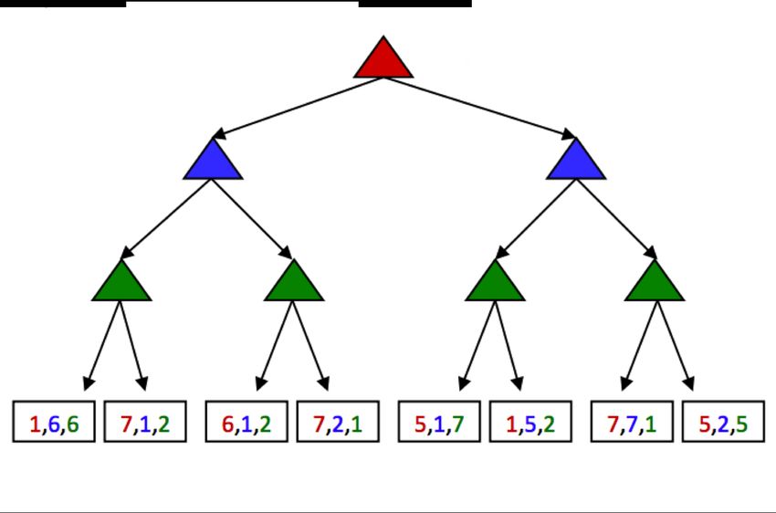
All of the world champion agents above use, at least to some degree, the adversarial search techniques that
we’re about to cover. As opposed to normal search, which returned a comprehensive plan, adversarial search
returns a strategy, or policy, which simply recommends the best possible move given some configuration of
our agent(s) and their adversaries. We’ll soon see that such algorithms have the beautiful property of giving
rise to behavior through computation - the computation we run is relatively simple in concept and widely
generalizable, yet innately generates cooperation between agents on the same team as well as "outthinking"
of adversarial agents.

Minimax
The first zero-sum-game algorithm we will consider is minimax, which runs under the motivating assump-
tion that the opponent we face behaves optimally, and will always perform the move that is worst for us. To
introduce this algorithm, we must first formalize the notion of terminal utilities and state value. The value
of a state is the optimal score attainable by the agent which controls that state. In order to get a sense of
what this means, observe the following trivially simple Pacman game board:

Assume that Pacman starts with 10 points and loses 1 point per move until he eats the pellet, at which point
the game arrives at a terminal state and ends. We can start building a game tree for this board as follows,
where children of a state are successor states just as in search trees for normal search problems:

CS 188, Spring 2020, Note 3                                                                                2
It’s evident from this tree that if Pacman goes straight to the pellet, he ends the game with a score of 8 points,
whereas if he backtracks at any point, he ends up with some lower valued score. Now that we’ve generated
a game tree with several terminal and intermediary states, we’re ready to formalize the meaning of the value
of any of these states.
A state’s value is defined as the best possible outcome (utility) an agent can achieve from that state. We’ll
formalize the concept of utility more concretely later, but for now it’s enough to simply think of an agent’s
utility as its score or number of points it attains. The value of a terminal state, called a terminal utility, is
always some deterministic known value and an inherent game property. In our Pacman example, the value
of the rightmost terminal state is simply 8, the score Pacman gets by going straight to the pellet. Also, in this
example, the value of a non-terminal state is defined as the maximum of the values of its children. Defining
V (s) as the function defining the value of a state s, we can summarize the above discussion:

       ∀ non-terminal states, V (s) =          max            V (s0 )
                                          s0 ∈successors(s)
            ∀ terminal states, V (s) =       known

This sets up a very simple recursive rule, from which it should make sense that the value of the root node’s
direct right child will be 8, and the root node’s direct left child will be 6, since these are the maximum
possible scores the agent can obtain if it moves right or left, respectively, from the start state. It follows that
by running such computation, an agent can determine that it’s optimal to move right, since the right child
has a greater value than the left child of the start state.
Let’s now introduce a new game board with an adversarial ghost that wants to keep Pacman from eating the
pellet.

The rules of the game dictate that the two agents take turns making moves, leading to a game tree where
the two agents switch off on layers of the tree that they "control". An agent having control over a node
simply means that node corresponds to a state where it is that agent’s turn, and so it’s their opportunity to
decide upon an action and change the game state accordingly. Here’s the game tree that arises from the new
two-agent game board above:

CS 188, Spring 2020, Note 3                                                                                      3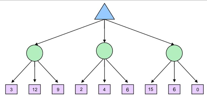
Blue nodes correspond to nodes that Pacman controls and can decide what action to take, while red nodes
correspond to ghost-controlled nodes. Note that all children of ghost-controlled nodes are nodes where the
ghost has moved either left or right from its state in the parent, and vice versa for Pacman-controlled nodes.
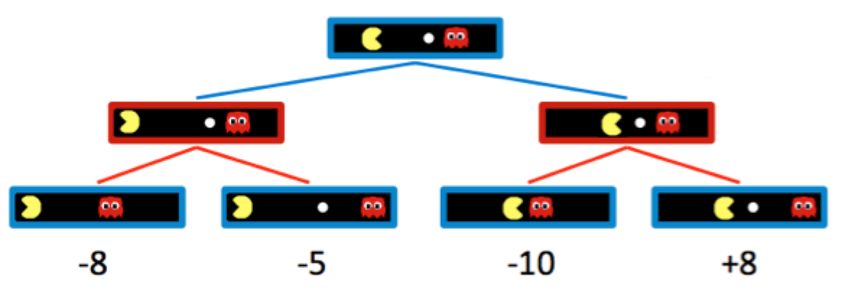
For simplicity purposes, let’s truncate this game tree to a depth-2 tree, and assign spoofed values to terminal
states as follows:
Naturally, adding ghost-controlled nodes changes the move Pacman believes to be optimal, and the new
optimal move is determined with the minimax algorithm. Instead of maximizing the utility over children
at every level of the tree, the minimax algorithm only maximizes over the children of nodes controlled by
Pacman, while minimizing over the children of nodes controlled by ghosts. Hence, the two ghost nodes
above have values of min(−8, −5) = −8 and min(−10, +8) = −10 respectively. Correspondingly, the root
node controlled by Pacman has a value of max(−8, −10) = −8. Since Pacman wants to maximize his score,
he’ll go left and take the score of −8 rather than trying to go for the pellet and scoring −10. This is a prime
example of the rise of behavior through computation - though Pacman wants the score of +8 he can get if he
ends up in the rightmost child state, through minimax he "knows" that an optimally-performing ghost will
not allow him to have it. In order to act optimally, Pacman is forced to hedge his bets and counterintuitively
move away from the pellet to minimize the magnitude of his defeat. We can summarize the way minimax
assigns values to states as follows:
∀ agent-controlled states, V (s) = max V (s0 )
s0 ∈successors(s)
∀ opponent-controlled states, V (s) = min V (s0 )
s0 ∈successors(s)
∀ terminal states, V (s) = known
In implementation, minimax behaves similarly to depth-first search, computing values of nodes in the same
order as DFS would, starting with the the leftmost terminal node and iteratively working its way rightwards.
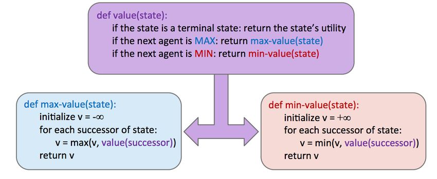
More precisely, it performs a postorder traversal of the game tree. The resulting pseudocode for minimax
is both elegant and intuitively simple, and is presented below:
CS 188, Spring 2020, Note 3 4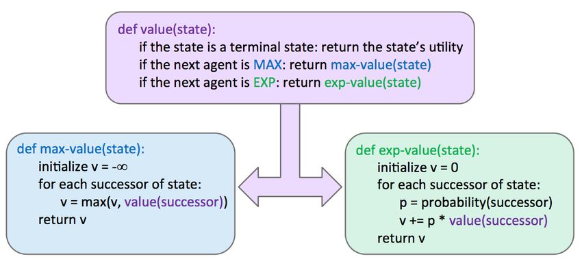
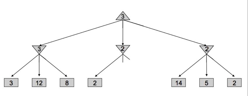
Alpha-Beta Pruning
Minimax seems just about perfect - it’s simple, it’s optimal, and it’s intuitive. Yet, its execution is very
similar to depth-first search and it’s time complexity is identical, a dismal O(bm ). Recalling that b is the
branching factor and m is the approximate tree depth at which terminal nodes can be found, this yields
far too great a runtime for many games. For example, chess has a branching factor b ≈ 35 and tree depth
m ≈ 100. To help mitigate this issue, minimax has an optimization - alpha-beta pruning.
Conceptually, alpha-beta pruning is this: if you’re trying to determine the value of a node n by looking at its
successors, stop looking as soon as you know that n’s value can at best equal the optimal value of n’s parent.
Let’s unravel what this tricky statement means with an example. Consider the following game tree, with
square nodes corresponding to terminal states, downward-pointing triangles corresponding to minimizing
nodes, and upward-pointing triangles corresponding to maximizer nodes:

Let’s walk through how minimax derived this tree - it began by iterating through the nodes with val-
ues 3, 12, and 8, and assigning the value min(3, 12, 8) = 3 to the leftmost minimizer. Then, it assigned
min(2, 4, 6) = 2 to the middle minimizer, and min(14, 5, 2) = 2 to the rightmost minimizer, before finally as-
signing max(3, 2, 2) = 3 to the maximizer at the root. However, if we think about this situation, we can come
to the realization that as soon as we visit the child of the middle minimizer with value 2, we no longer need
to look at the middle minimizer’s other children. Why? Since we’ve seen a child of the middle minimizer
with value 2, we know that no matter what values the other children hold, the value of the middle minimizer
can be at most 2. Now that this has been established, let’s think one step further still - the maximizer at
the root is deciding between the value of 3 of the left minimizer, and the value that’s ≤ 2, it’s guaranteed to
prefer the 3 returned by the left minimizer over the value returned by the middle minimizer, regardless of
the values of its remaining children. This is precisely why we can prune the search tree, never looking at
the remaining children of the middle minimizer:

CS 188, Spring 2020, Note 3                                                                                  5
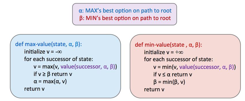
Implementing such pruning can reduce our runtime to as good as O(bm/2 ), effectively doubling our "solv-
able" depth. In practice, it’s often a lot less, but generally can make it feasible to search down to at least
one or two more levels. This is still quite significant, as the player who thinks 3 moves ahead is favored to
win over the player who thinks 2 moves ahead. This pruning is exactly what the minimax algorithm with
alpha-beta pruning does, and is implemented as follows:

Take some time to compare this with the pseudocode for vanilla minimax, and note that we can now return
early without searching through every successor.

Evaluation Functions
Though alpha-beta pruning can help increase the depth for which we can feasibly run minimax, this still
usually isn’t even close to good enough to get to the bottom of search trees for a large majority of games.
As a result, we turn to evaluation functions, functions that take in a state and output an estimate of the
true minimax value of that node. Typically, this is plainly interpreted as "better" states being assigned
higher values by a good evaluation function than "worse" states. Evaluation functions are widely employed
in depth-limited minimax, where we treat non-terminal nodes located at our maximum solvable depth
as terminal nodes, giving them mock terminal utilities as determined by a carefully selected evaluation
function. Because evaluation functions can only yield estimates of the values of non-terminal utilities, this
removes the guarantee of optimal play when running minimax.
A lot of thought and experimentation is typically put into the selection of an evaluation function when
designing an agent that runs minimax, and the better the evaluation function is, the closer the agent will come
to behaving optimally. Additionally, going deeper into the tree before using an evaluation function also tends
to give us better results - burying their computation deeper in the game tree mitigates the compromising
of optimality. These functions serve a very similar purpose in games as heuristics do in standard search
problems.

CS 188, Spring 2020, Note 3                                                                                  6
The most common design for an evaluation function is a linear combination of features.

                                Eval(s) = w1 f1 (s) + w2 f2 (s) + ... + wn fn (s)

Each fi (s) corresponds to a feature extracted from the input state s, and each feature is assigned a corre-
sponding weight wi . Features are simply some element of a game state that we can extract and assign a
numerical value. For example, in a game of checkers we might construct an evaluation function with 4 fea-
tures: number of agent pawns, number of agent kings, number of opponent pawns, and number of opponent
kings. We’d then select appropriate weights based loosely on their importance. In our checkers example, it
makes most sense to select positive weights for our agent’s pawns/kings and negative weights for our oppo-
nents pawns/kings. Furthermore, we might decide that since kings are more valuable pieces in checkers than
pawns, the features corresponding to our agent’s/opponent’s kings deserve weights with greater magnitude
than the features concerning pawns. Below is a possible evaluation function that conforms to the features
and weights we’ve just brainstormed:

      Eval(s) = 2 · agent_kings(s) + agent_pawns(s) − 2 · opponent_kings(s) − opponent_pawns(s)

As you can tell, evaluation function design can be quite free-form, and don’t necessarily have to be linear
functions either. The most important thing to keep in mind is that the evaluation function yields higher
scores for better positions as frequently as possible. This may require a lot of fine-tuning and experimenting
on the performance of agents using evaluation functions with a multitude of different features and weights.

Expectimax
We’ve now seen how minimax works and how running full minimax allows us to respond optimally against
an optimal opponent. However, minimax has some natural constraints on the situations to which it can re-
spond. Because minimax believes it is responding to an optimal opponent, it’s often overly pessimistic in
situations where optimal responses to an agent’s actions are not guaranteed. Such situations include scenar-
ios with inherent randomness such as card or dice games or unpredictable opponents that move randomly
or suboptimally. We’ll talk about scenarios with inherent randomness much more in detail when we discuss
Markov decision processes in the next note.
This randomness can be represented through a generalization of minimax known as expectimax. Expecti-
max introduces chance nodes into the game tree, which instead of considering the worst case scenario as
minimizer nodes do, considers the average case. More specifically, while minimizers simply compute the
minimum utility over their children, chance nodes compute the expected utility or expected value. Our rule
for determining values of nodes with expectimax is as follows:

       ∀ agent-controlled states, V (s) =         max            V (s0 )
                                             s0 ∈successors(s)

                 ∀ chance states, V (s) =          ∑             p(s0 |s)V (s0 )
                                             s0 ∈successors(s)
                ∀ terminal states, V (s) =      known

In the above formulation, p(s0 |s) refers to either the probability that a given nondeterministic action results
in moving from state s to s0 , or the probability that an opponent chooses an action that results in moving
from state s to s0 , depending on the specifics of the game and the game tree under consideration. From this
definition, we can see that minimax is simply a special case of expectimax. Minimizer nodes are simply
chance nodes that assign a probability of 1 to their lowest-value child and probability 0 to all other children.

CS 188, Spring 2020, Note 3                                                                                   7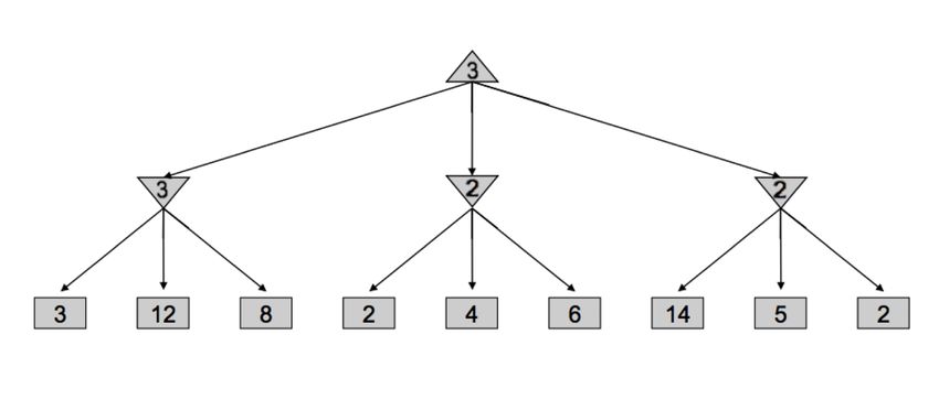
In general, probabilities are selected to properly reflect the game state we’re trying to model, but we’ll cover
how this process works in more detail in future notes. For now, it’s fair to assume that these probabilities
are simply inherent game properties.
The pseudocode for expectimax is quite similar to minimax, with only a few small tweaks to account for
expected utility instead of minimum utility, since we’re replacing minimizing nodes with chance nodes:

Before we continue, let’s quickly step through a simple example. Consider the following expectimax tree,
where chance nodes are represented by circular nodes instead of the upward/downward facing triangles for
maximizers/minimizers.

Assume for simplicity that all children of each chance node have a probability of occurrence of 13 . Hence,
from our expectimax rule for value determination, we see that from left to right the 3 chance nodes take on
values of 13 · 3 + 13 · 12 + 13 · 9 = 8 , 13 · 2 + 13 · 4 + 13 · 6 = 4 , and 31 · 15 + 13 · 6 + 13 · 0 = 7 . The maximizer
selects the maximimum of these three values, 8 , yielding a filled-out game tree as follows:

CS 188, Spring 2020, Note 3                                                                                             8
As a final note on expectimax, it’s important to realize that, in general, it’s necessary to look at all the
children of chance nodes – we can’t prune in the same way that we could for minimax. Unlike when
computing minimums or maximums in minimax, a single value can skew the expected value computed by
expectimax arbitrarily high or low. However, pruning can be possible when we have known, finite bounds
on possible node values.

Mixed Layer Types
Though minimax and expectimax call for alternating maximizer/minimizer nodes and maximizer/chance
nodes respectively, many games still don’t follow the exact pattern of alternation that these two algorithms
mandate. Even in Pacman, after Pacman moves, there are usually multiple ghosts that take turns making
moves, not a single ghost. We can account for this by very fluidly adding layers into our game trees as
necessary. In the Pacman example for a game with four ghosts, this can be done by having a maximizer
layer followed by 4 consecutive ghost/minimizer layers before the second Pacman/maximizer layer. In fact,
doing so inherently gives rise to cooperation across all minimizers, as they alternatively take turns further
minimizing the utility attainable by the maximizer(s). It’s even possible to combine chance node layers with
both minimizers and maximizers. If we have a game of Pacman with two ghosts, where one ghost behaves
randomly and the other behaves optimally, we could simulate this with alternating groups of maximizer-
chance-minimizer nodes.

As is evident, there’s quite a bit of room for robust variation in node layering, allowing development of
game trees and adversarial search algorithms that are modified expectimax/minimax hybrids for any zero-
sum game.

CS 188, Spring 2020, Note 3                                                                                9
General Games
Not all games are zero-sum. Indeed, different agents may have have distinct tasks in a game that don’t
directly involve strictly competing with one another. Such games can be set up with trees characterized by
multi-agent utilities. Such utilities, rather than being a single value that alternating agents try to minimize or
maximize, are represented as tuples with different values within the tuple corresponding to unique utilities
for different agents. Each agent then attempts to maximize their own utility at each node they control,
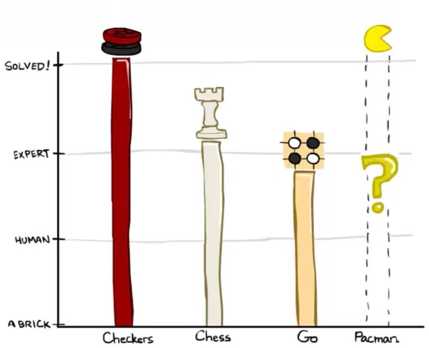
ignoring the utilities of other agents. Consider the following tree:
The red, green, and blue nodes correspond to three separate agents, who maximize the red, green, and blue
utilities respectively out of the possible options in their respective layers. Working through this example
ultimately yields the utility tuple (5, 2, 5) at the top of the tree. General games with multi-agent utilities are
a prime example of the rise of behavior through computation, as such setups invoke cooperation since the
utility selected at the root of the tree tends to yield a reasonable utility for all participating agents.
Utilities
Thoughout our discussion of games, the concept of utility has come up repeatedly. Utility values are gener-
ally hard-wired into games, and agents run some variation of the algorithms discussed in this note to select
an action. We’ll now discuss what’s necessary in order to generate a viable utility function.
Rational agents must follow the principle of maximum utility - they must always select the action that
maximizes their expected utility. However, obeying this principle only benefits agents that have rational
preferences. To construct an example of irrational preferences, say there exist 3 objects, A, B, and C, and
our agent is currently in possession of A. Say our agent has the following set of irrational preferences:
• Our agent prefers B to A plus $1
• Our agent prefers C to B plus $1
• Our agent prefers A to C plus $1
CS 188, Spring 2020, Note 3 10A malicious agent in possession of B and C can trade our agent B for A plus a dollar, then C for B plus a
dollar, then A again for C plus a dollar. Our agent has just lost $3 for nothing! In this way, our agent can be
forced to give up all of its money in an endless and nightmarish cycle.
Let’s now properly define the mathematical language of preferences:
• If an agent prefers receiving a prize A to receiving a prize B, this is written A B
• If an agent is indifferent between receiving A or B, this is written as A ∼ B
• A lottery is a situation with different prizes resulting with different probabilities. To denote lottery
where A is received with probability p and B is received with probability (1 − p), we write
L = [p, A; (1 − p), B]
In order for a set of preferences to be rational, they must follow the five Axioms of Rationality:
• Orderability: (A B) ∨ (B A) ∨ (A ∼ B)
A rational agent must either prefer one of A or B, or be indifferent between the two.
• Transitivity: (A B) ∧ (B C) ⇒ (A C)
If a rational agent prefers A to B and B to C, then it prefers A to C.
• Continuity: A B C ⇒ ∃p [p, A; (1 − p), C] ∼ B
If a rational agent prefers A to B but B to C, then it’s possible to construct a lottery L between A
and C such that the agent is indifferent between L and B with appropriate selection of p.
• Substitutability: A ∼ B ⇒ [p, A; (1 − p), C] ∼ [p, B; (1 − p), C]
A rational agent indifferent between two prizes A and B is also indifferent between any two
lotteries which only differ in substitutions of A for B or B for A.
• Monotonicity: A B ⇒ (p ≥ q ⇔ [p, A; (1 − p), B] [q, A; (1 − q), B]
If a rational agent prefers A over B, then given a choice between lotteries involving only A and B,
the agent prefers the lottery assigning the highest probability to A.
If all five axioms are satisfied by an agent, then it’s guaranteed that the agent’s behavior is describable as
a maximization of expected utility. More specifically, this implies that there exists a real-valued utility
function U that when implemented will assign greater utilities to preferred prizes, and also that the utility
of a lottery is the expected value of the utility of the prize resulting from the lottery. These two statements
can be summarized in two concise mathematical equivalences:
U(A) ≥ U(B) ⇔ A B (1)
U([p1 , S1 ; ... ; pn , Sn ]) = ∑ piU(Si ) (2)
i
If these constraints are met and an appropriate choice of algorithm is made, the agent implementing such
a utility function is guaranteed to behave optimally. Let’s discuss utility functions in greater detail with a
concrete example. Consider the following lottery:
L = [0.5, $0; 0.5, $1000]
CS 188, Spring 2020, Note 3 11This represents a lottery where you receive $1000 with probability 0.5 and $0 with probability 0.5. Now
√
consider three agents A1 , A2 , and A3 which have utility functions U1 ($x) = x, U2 ($x) = x, and U3 ($x) = x2
respectively. If each of the three agents were faced with a choice between participting in the lottery and
receiving a flat payment of $500, which would they choose? The respective utilities for each agent of
participating in the lottery and accepting the flat payment are listed in the following table:
Agent Lottery Flat Payment
1 500 500
2 15.81 22.36
3 500000 250000
These utility values for the lotteries were calculated as follows, making use of equation (2) above:
U1 (L) = U1 ([0.5, $0; 0.5, $1000]) = 0.5 ·U1 ($1000) + 0.5 ·U1 ($0) = 0.5 · 1000 + 0.5 · 0 = 500
√ √
U2 (L) = U2 ([0.5, $0; 0.5, $1000]) = 0.5 ·U2 ($1000) + 0.5 ·U2 ($0) = 0.5 · 1000 + 0.5 · 0 = 15.81
U3 (L) = U1 ([0.5, $0; 0.5, $1000]) = 0.5 ·U3 ($1000) + 0.5 ·U3 ($0) = 0.5 · 10002 + 0.5 · 02 = 500000
With these results, we can see that agent A1 is indifferent between participating in the lottery and receiving
the flat payment (the utilities for both cases are identical). Such an agent is known as risk-neutral. Similarly,
agent A2 prefers the flat payment to the lottery and is known as risk-averse and agent A3 prefers the lottery
to the flat payment and is known as risk-seeking.
Summary
In this note, we shifted gears from considering standard search problems where we simply attempt to find a
path from our starting point to some goal, to considering adversarial search problems where we may have
opponents that attempt to hinder us from reaching our goal. Two primary algorithms were considered:
• Minimax - Used when our opponent(s) behaves optimally, and can be optimized using α-β pruning.
Minimax provides more conservative actions than expectimax, and so tends to yield favorable results
when the opponent is unknown as well.
• Expectimax - Used when we facing a suboptimal opponent(s), using a probability distribution over
the moves we believe they will make to compute the expectated value of states.
In most cases, it’s too computationally expensive to run the above algorithms all the way to the level of
terminal nodes in the game tree under consideration, and so we introduced the notion of evaluation functions
for early termination. Finally, we considered the problem of defining utility functions for agents such that
they make rational decisions. With appropriate function selection, we can additionally make our agents
risk-seeking, risk-averse, or risk-neutral.
CS 188, Spring 2020, Note 3 12You can also read