CUBETR: LEARNING TO SOLVE THE RUBIK'S CUBE USING TRANSFORMERS - OpenReview
←
→
Page content transcription
If your browser does not render page correctly, please read the page content below
Under review as a conference paper at ICLR 2022

C UBE TR: L EARNING TO S OLVE                                   THE       RUBIK ’ S C UBE
USING T RANSFORMERS

 Anonymous authors
 Paper under double-blind review

                                            A BSTRACT

         Since its first appearance, transformers have been successfully used in wide rang-
         ing domains from computer vision to natural language processing. Application of
         transformers in Reinforcement Learning by reformulating it as a sequence mod-
         elling problem was proposed only recently. Compared to other commonly ex-
         plored reinforcement learning problems, the Rubik’s cube poses a unique set of
         challenges. The Rubik’s cube has a single solved state for quintillions of possible
         configurations which leads to extremely sparse rewards. The proposed model Cu-
         beTR attends to longer sequences of actions and addresses the problem of sparse
         rewards. CubeTR learns how to solve the Rubik’s cube from arbitrary starting
         states without any human prior, and after move regularisation, the lengths of so-
         lutions generated by it are expected to be very close to those given by algorithms
         used by expert human solvers. CubeTR provides insights to the generalisability
         of learning algorithms to higher dimensional cubes and the applicability of trans-
         formers in other relevant sparse reward scenarios.

1   I NTRODUCTION

Originally proposed by Vaswani et al. (2017), transformers have gained a lot of attention over the
last few years. Transformers are widely used for sequence to sequence learning in NLP (Radford
et al., 2018; Devlin et al., 2019; Radford et al., 2019; Brown et al., 2020), and start to show promises
in other domains like image to classification (Dosovitskiy et al., 2020), instance segmentation (Wang
et al., 2021) in computer vision and the decision transformer (Chen et al., 2021) in reinforcement
learning. Transformers are capable of modeling long-range dependencies, and have tremendous
representation power. In particular, the core mechanism of Transformers, self-attention, is designed
to learn and update features based on all pairwise similarities between individual components of
a sequence. There have been great advances of the transformer architecture in the field of natural
language processing, with models like GPT-3 (Brown et al., 2020) and BERT (Devlin et al., 2019),
and drawing upon transformer block architectures designed in this domain has proven to be very
effective in other domains as well.
Although transformers have become widely used in NLP and Computer Vision, its applications in
Reinforcement Learning are still under-explored. Borrowing form well experimented and easily
scalable architectures like GPT (Radford et al., 2018), exploring applications of transformers in
other domains has started becoming easier. The use of transformers in core reinforcement learning
was first proposed by Chen et al. (2021). Reformulating the reinforcement learning objective as
learning of action sequences, they used transformers to generate the action sequence, i.e. the policy.
Reinforcement Learning is a challenging domain. Contrary to other learning paradigms like super-
vised, unsupervised and self-supervised, reinforcement learning involves learning an optimal policy
for an agent interacting with its environment. Rather than minimising losses with the expected
output, reinforcement learning approaches involve maximising the reward. Training deep reinforce-
ment learning (Mousavi et al., 2016) architectures has been notoriously difficult, and the learning
algorithm is unstable or even divergent when action value function is approximated with a nonlinear
function like the activation functions common-place in neural networks. Various algorithms like
DQN (Mnih et al., 2013) and D-DQN (Van Hasselt et al., 2016) tackle some of these challenges
involved with deep reinforcement learning.

                                                   1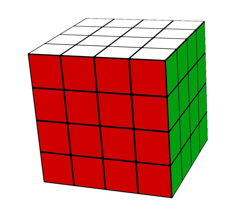
Under review as a conference paper at ICLR 2022

                              No Reward!

                                                                                           Reward 1

       State i1         State i2           State i3         State i4                      Solved State

Figure 1: Sparse rewards in the case of the Rubik’s cube. The state space is extremely large, but
only the final solved state has a non-zero reward, making the reward distribution extremely sparse.

Reinforcement learning has seen applications in learning many games like chess, shogi (Silver et al.,
2017), hex (Young et al., 2016) and Go (Silver et al., 2018). In October 2015, the distributed version
of AlphaGo (Silver et al., 2016) defeated the European Go champion, becoming the first computer
Go program to have beaten a professional human player on a full-sized board without handicap.
Reinforcement learning has also been used for solving different kinds of puzzles (Dandurand et al.,
2012), for protein folding (Jumper et al., 2021), for path planning (Zhang et al., 2015) and many
other applications.
The Rubik’s Cube is a particularly challenging single player game, invented in 1974 by Hungarian
architecture and design professor Erno Rubik. Starting from a single solved state, the simple 3×3
rubik’s cube can end up in 43 quintillion (43×1018 ) different configurations. The number of different
configurations (God’s number) for a modified 4×4 cube is not even known. Thus, a random set of
moves from this tremendous state space is highly unlikely to end up in the solved space. It is a marvel
that humans have devised algorithms that can solve this challenging puzzle from any configuration
in bounded number of moves.
Computers have been able to solve the cube for a long time now (Korf, 1982). By implementing in
software, an algorithm used by humans, very simple programs can be created to solve the cube very
efficiently. These algorithms are, however, deeply rooted in group theory. Enabling an algorithm to
learn to solve the cube on its own, without human priors is a much more challenging task. With its
inherent complexity, this problem can provide new insights into much harder reinforcement learning
problems, while also presenting new applications and interpretations of machine learning in abstract
subjects like group theory and basic maths.
One of the biggest challenges in solving the Rubik’s cube using reinforcement learning is that of
sparse rewards. Since there is a single solved state, there is a single state with a non zero reward.
All other 43 quintillion - 1 states have no reward. Reinforcement learning algorithms that rely very
heavily on the rewards to decide optimal policies suffer since even large action sequences may end
up with no reward. The method proposed in this paper should be easy to generalise to many other
problems suffering with sparse rewards, and may help provide deeper insights of the usefulness of
transformers in more complicated reinforcement learning tasks. Although there have been some
works solving this problem using deep reinforcement learning, this work also provides insights into
the relationship between reinforcement learning policies and natural language processing sequential
data generation.
This work is the first to explore the use of transformers in solving the rubik’s cube, or in general
any sparse reward reinforcement learning scenarios. It is also the first one to consider higher dimen-
sional1 cubes. Improving upon the decision transformer, CubeTR is able to effectively propagate
the reward to actions far away from the final goal state. The transformer is further biased to gener-
ate smaller solutions by using a move regularisation factor. This is done to allow it to learn more
efficient solutions, bridging the gap to human algorithms.

    1
      Note that here and everywhere else in the paper, higher dimensional does not mean more dimensions, but
rather larger scales in each dimension (eg: 4×4×4 instead of 3×3×3, and not 3×3×3×3)

                                                      2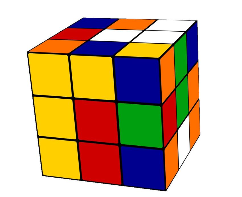
Under review as a conference paper at ICLR 2022

In the next section, some past work related to transformers, algorithms used for solving the rubik’s
cube and in general reinforcement learning are discussed. The methodology used in CubeTR is dis-
cussed in Section 3, along with description of the cube’s representation. The experimental results of
CubeTR and its comparison with other human based algorithms is discussed in Section 4, followed
by the conclusions in Section 5.

2      R ELATED W ORK
Transformers were first proposed by Vaswani et al. (2017), where they worked with machine transla-
tion, but later apply it to constituency parsing to demonstrate the generalisability of the transformer
architecture. Consisting of only attention blocks, the authors demonstrate that the transformer can
replace recurrence and convolutions entirely. Along with superior performance, they demonstrated
that transformers also lead to lower resource requirements, with more parallelizability. They laid the
foundations for many subsequent works in NLP (Radford et al., 2018; Devlin et al., 2019; Radford
et al., 2019; Brown et al., 2020) as well as computer vision (Dosovitskiy et al., 2020).
In GPT (Radford et al., 2018) the process of generative pre-training was first proposed. They showed
that pre-training on a large scale unlabelled dataset gives significant performance boost over previous
methods. Many other works have experimented with and adopted this approach, including GPT-2
(Radford et al., 2019) and GPT-3 (Brown et al., 2020). In (Hu et al., 2020), the GPT architecture was
applied to graph neural networks. The GPT-2 architecture has been used for applications like data
augmentation (Papanikolaou & Pierleoni, 2020) as well. The recently proposed GPT-3 architecture
had taken the NLP community by storm, and has also seen many applications. Elkins & Chun
(2020) even experimented with whether GPT-3 can pass the writer’s Turing’s test. The Decision
Transformer (Chen et al., 2021), the first work to propose the use of transformers in reinforcement
leanrnig, also uses the GPT-3 architecture.

            Natural Language Processing            Computer Vision                 Reinforcement Learning

                           それ は とてもかっこいい                                   Encoder Block                action
     Encoder Block                                       Encoder Block
                                             MLP
                             Decoder Block                                 Encoder Block            Decoder Block
     Encoder Block                                       Encoder Block
                                             Cat
                             Decoder Block                                 Encoder Block            Decoder Block
     Encoder Block                                       Encoder Block

                             Decoder Block                                                          Decoder Block

                                                                         state action reward
    it is so very cool

Figure 2: Some applications of transformers in different fields of machine learning. For NLP, a
machine translation pipeline is show, while for CV, the vision transformer (Dosovitskiy et al., 2020)
pipeline is shown. The decision transformer (Chen et al., 2021) is shown for RL.

Reinforcement Learning has been gaining a lot of popularity in recent times. With the advent of deep
reinforcement learning, many other methods have been proposed in this field. Deep Q-Learning
(Mnih et al., 2013; Hausknecht & Stone, 2015; Wang et al., 2016; Hessel et al., 2018) is a natural
extension to the vanilla Q-learning algorithm where a neural network is used to predict the expected
reward for each action from a particular state. Policy gradients (Schulman et al., 2015a; Mnih et al.,
2016; Schulman et al., 2015b) uses gradient descent and other optimisation algorithms on the policy
space to find optimal policies. Value iteration (Jothimurugan et al., 2021; Ernst et al., 2005; Munos,
2005) is another popular approach, where the expected value of each state is either calculated or
approximated. The value of a state is the maximum reward that can be obtained from that state
using some optimal policy. The multi-armed bandit (Vermorel & Mohri, 2005; Auer et al., 2002)
problem is a classic example of the exploration vs exploitation dilemma, and many reinforcement
learning algorithms have been proposed to address it (Villar et al., 2015; Liu & Zhao, 2010).
A typical situation for reinforcement learning is a situation where an agent has to reach a goal and
only receives a positive reward signal when he either reaches or is close enough to the target. This

                                                          3
Under review as a conference paper at ICLR 2022

situation of sparse rewards is challenging for usual reinforcement learning that depend too much on
the rewards to decide exploration and policies. Several methods have been proposed to deal with
sparse reward situations (Riedmiller et al., 2018; Trott et al., 2019). Curiosity driven approaches
(Pathak et al., 2017; Burda et al., 2018; Oudeyer, 2018) use curiosity as an intrinsic reward signal
to enable the agent to explore its environment and learn skills that might be useful later in its life.
Curriculum learning methods (Florensa et al., 2018) use a generative approach to getting new or
auxiliary tasks that the agent solves. Reward Shaping (Mataric, 1994; Ng et al., 1999) is another
commonly used approach in which the primary reward of the environment is enhanced with some
additional reward features.
The use of transformers in reinforcement learning was first proposed by Chen et al. (2021). Ab-
stracting reinforcement learning as a sequence modeling problem, the decision transformer simply
outputs the optimal actions. By conditioning an autoregressive model on the desired reward, past
states, and actions, the decision transformer model can generate future actions that achieve the de-
sired reward. Despite its simplicity, it obtained impressive results. However, it posed challenges in
reinforcement learning problems like the Rubik’s cube, where the past actions and states may not
affect future actions significantly. The decision transformer showed promise in the sparse reward
scenario, since it makes no assumption on the density of rewards.
Solving the rubik’s cube using reinforcement learning is a relatively under explored field. El-Sourani
et al. (2010) proposed an evolutionary algorithm using domain knowledge and group theoretic argu-
ments. Brunetto & Trunda (2017) attempted to train a deep learning model to act as an alternative
heuristic for searching the rubik’s cube’s solution space. The search algorithm, however, takes an
extraordinarily long time to run. McAleer et al. (2018) used approximate policy iteration and trained
on a distribution of states that allows the reward to propagate from the goal state to states farther
away. Another deep reinforcement learning method was proposed recently (Agostinelli et al., 2019)
that learns how to solve increasingly difficult states in reverse from the goal state without any specific
domain knowledge. The approach of CubeTR is most similar to this work, and draws inspiration
from it. Leveraging the representation power of transformers, CubeTR also explores generalisation
to higher dimensional cubes.
Humans have been able to solve for a long time, with many different algorithms developed (Kunkle
& Cooperman, 2007; Korf, 1982; Rokicki et al., 2014). One of the most popular and efficient
algorithms is Kociemba (Rokicki et al., 2014; Aqra & Abu Salah, 2017). Using concepts of group
theory, the method reduces the problem by maneuvering the cube to smaller sub-groups, eventually
leading to the solved state. Thistlethwaite’s algorithm and Korf’s algorithm are some other similar
group theoretic approaches. Besides these group theoretic and computational approaches, there have
been many comparatively simpler algorithms as well (Nourse, 1981), that can be used by humans
to solve the cube easily. With intuition and practice, humans are able to solve this combinatorial
monster surprisingly efficiently and extremely fast, with the world record being 3.47 seconds.

3     P ROPOSED M ETHODOLOGY

The proposed method CubeTR involves three parts. First an appropriate representation of the cube’s
state and the choice of rewards needs to be considered. With the encoded cubes, the model is then
trained. Finally, the actual solution to the cube is extracted from the model, and decoded back to
human readable format. In what follows, each of these stages are described in detail.

3.1   R EPRESENTATION

The 3×3 cube, perhaps the most commonly used and easiest version of the rubik’s cube, is itself a
complicated structure. Being a three dimensional puzzle with 26 colored pieces, 6 colors, and three
distinct types of pieces, an appropriate representation that captures the inherent patterns in the cube
is of utmost importance to facilitate proper learning. Human solvers usually use shorthand notations
like replacing colors and moves with their initials. A commonly used notation for describing cube
solving algorithms is the ‘singmaster notation’, where moves are denoted by the faces, while the
direction of the move is denoted by an additional prime symbol (for example, F means a move that
rotates the front face in clock wise direction, while F’ means anti-clockwise direction).

                                                    4
Under review as a conference paper at ICLR 2022
Another major consideration while deciding a representation for a state of the cube is that of gener-
alisability to higher dimensions. A representation that can be used for cubes of higher dimensions
as well will be most ideal because it will allow an easy and efficient adaptation of learning strategies
across the domains. Although the action space is very different, with the number of possible actions
changing in proportion with the dimension, the state space can be mapped to an identical represen-
tation space. Besides better generalisability, it also allows a more uniform and reusable pipeline for
different versions of the cube.
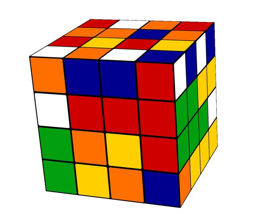
Figure 3: Representation of the rubik’s cube states. Examples of 3×3 and 4×4 are shown.
The proposed representation scheme can be thought of as flattening out the cube into a 2d image.
Except the back face center pieces, all individual pieces in the cube correspond to a single square
region of color in the encoded image. For pieces that have two or three colored sides, the square
region is filled with a color that is the mean of all these colors. For easier calculations, the image
was taken to be 700×700, so that each region for the 3×3 is of size 100×100, while that for the
4×4 is 70×70 pixels. A 2D image was chosen instead of a 1D vector representation to avoid the loss
of too much information in the encoding step itself. Note that the colors of the individual regions
along with their positional encodings (as used in transformers), are sufficient to completely describe
a given state.
The rewards also need to be chosen wisely for effective learning. The true reward is 1 for the solved
state and 0 for all other states. There is no notion of undesirable states in the rubik’s cube, so there
are no negative rewards. Now for obtaining the optimal policy, a different set of pseudo rewards
are used. These pseudo rewards are also predicted by the transformer model, and are used for move
regularisation, as described in later sections. The pseudo-reward is:
α
R0 = (1)
1+η
where η is the expected number of moves to solution (explained later), and α is a tunable hyperpa-
rameter. In practiice, α = 1 was used. Note that with this setting, the fully solved state has R’ =
1, and all other states have rewards 0 < R0 < 1. States with larger expected number of moves to
solution have a lower pseudo reward and vice versa.
3.2 T RAINING
During the training phase, CubeTR is effectively a reversed cascaded decision transformer with
modifications similar to the vision transformer. This structure is proposed to better model the specific
properties of the Rubik’s cube. Firstly, instead of some previous state-action-reward pairs, only the
present state is passed as the input to the causal transformer. This is because the rubik’s cube
is memoryless, and the optimal solution from a particular state does not depend on past states or
actions. The encoded image of the state was passed to the transformer in an identical manner as the
vision transformer (Dosovitskiy et al., 2020). Again, similar to the vision transformer, the outputs of
the decoder are passed through a double headed densely connected neural network, and the pseudo
5
Under review as a conference paper at ICLR 2022

reward R’ and the next action are obtained from that. The pseudo reward is trained using regression
loss, while the action is trained using classification loss.

                             Training Pipeline                                             Decision Block                               Transformer Block

                 Lact               Lact                 Lact
                                                                                               Transformer Block
                                                                                                                                                 Encoder Block

       a         R’            a     R’             a     R’                      Pseudo
                                                                                                                                  MLP
                                                                                  Reward
                                                                                                                                                 Encoder Block
                                                                                                                          Next      Pseudo
                                                                                   Next
                                                                                                                         Action     Reward
       Decision                Decision             Decision                      Action
        Block                   Block                Block                                                                                       Encoder Block
                                                                                                Representation

                        a3                  a2                    a1

                      Move 3               Move 2               Move 1

           R3’                     R2’                  R1’                                          state

Figure 4: The training pipeline and principal blocks used in CubeTR. Starting from the solved state,
the decision blocks are cascaded in reverse to get the ground truth for actions. In addition to Lact ,
there are two more losses, Lrew and Lmov , that have not been shown in the diagram for clarity.

The training pipeline proposed is visualised in Fig 4. Similar to the approach used by Agostinelli
et al. (2019), CubeTR starts training from the solved state, and makes moves from here to explore
the state space. While generating these moves, it is ensured that there are no cycles in the state space,
so that the same state is not visited multiple times. The process of generation of these states is thus,
fixed a priori, and the training phase can be considered as the exploration phase of the agent. The
reason for exploring the states in the reverse direction is that now, an estimate for the pseudo reward
is readily available. Perhaps more importantly, for any particular state, the last move in this reverse
process will be the next action in a possible solution. The model is trained using this as the action
label. The transformer block described in Fig 4 has very similar structure to the vision transformer
(Dosovitskiy et al., 2020) with a dual headed MLP instead to predict both action and pseudo reward.
Each action can only be one out of a set of possible actions. In the rubik’s cube, this set is simply
the set of all 90 degree face rotations. Thus, there are 12 possible actions (6 faces × 2 directions).
So, the problem of predicting the action is formulated as a classification task and the vanilla cross
entropy loss is used to train the action head. Since the pseudo reward is a real number between 0
and 1, and can take a larger number of continuous values, it is formulated as a regression task, and
the MSE loss is used to train the pseudo reward head. These two losses are, therefore,

                                            |A|
                                          m X                                                                        m
                                          X                   (i)          (i)                                    1 X (i)
                        Lact =                            âj log aj                               Lrew =               (r − r̂(i) )2                            (2)
                                           i=1 j=1
                                                                                                                 2m i=1

           (i)                                                                                                                                 (i)
where aj is the j th component of the predicted action for the ith example, and âj is the corre-
sponding label. A is the set of all actions, and |A| is the length of this set. r(i) and r̂(i) are the
predicted and labelled pseudo rewards respectively for the ith example. The total number of exam-
ples is m. In addition to the above two losses, a third loss is introduced to incentivise the model to
learn smaller solutions. This move regularisation loss is given by

                                                                                           m
                                                                                   1 X
                                                                         Lmov =          (α − r(i) )2                                                            (3)
                                                                                  2m i=1

where α is the same used in eq 1 and rest of the notation is the same as used in eq 2. The intuition
behind this loss is to penalise solutions that have a larger expected number of moves to reach the
solution. This is preferred over simply regularising the number of moves, since the variation of the
pseudo reward, as given by eq 1, is comparatively smoother, and in practice, this is easier to train.
The total loss is simply a weighted sum of the above three losses, with the relative weights being
tunable hyperparameters.

                                                                                           6
Under review as a conference paper at ICLR 2022

                                                                                                           Validate Action
      Validate            Validate            Validate            Validate
       Action              Action              Action              Action                                    N          a = random
                                                                                                                       (with prob p)
      a     R’            a    R’             a    R’             a    R’                        R’ >             Y
                                                                                               previous
                                                                                                 R’?
      Decision            Decision            Decision            Decision
       Block               Block               Block               Block                        N

                                                                                                   First         Y
                                                                                                                         Save R’
                   a                   a                   a                   a                   R’?

                 Move 1              Move 2              Move 3              Move n
      Starting                                                                        Solved
       state                                                                           state   a       R’                Return a

Figure 5: The inference pipeline used in CubeTR. Starting from an arbitrary unsolved state, new
actions are predicted, and performed, leading to the solved state. Validate Action is a simple logical
module that validates if the pseudo reward is increasing and if it is not, replaces the predicted action
with a random action.

3.3    I NFERENCE

During inference, the flow direction is forward, that is, from arbitrary starting states to the solved
state. As can be seen in Fig 5, the decision blocks trained earlier are used to predict action and
pseudo reward pairs. Each pair is first passed through the validate action block, and the action
returned by it is performed on the state to get to a new state. This process is repeater till the solved
state is reached. In practice, a maximum number of moves is allowed, to prevent crashes due to
infinite loops.
The validate action block is a simple logical module that checks if the pseudo reward is actually
increasing. If it is, this means that the predicted action takes the agent to a state closer to the
solution, and thus, the action is performed. If the pseudo reward is decreasing, a random action
is chosen with probability p, and the predicted action is still performed with probability 1-p. This
is to accommodate errors in the predicted pseudo reward. The random action chosen can help
in eliminating closed loops in the predicted actions. In practice, the check is done with a small
threshold, that is, Rn0 > Rn−1
                           0
                               − δ is checked instead of Rn0 > Rn−10
                                                                       .

3.4    D ISCUSSION

The rubik’s cube is a challenging and representationally complex puzzle. It is quite difficult to
capture the complex patterns involved in it. Predicting the optimal action using only the current
state often leads to underfitting, and almost uniform action predictions, which do not correspond to
actual solutions. However, the transformer has a great representation power, and CubeTR is able
to capture the complexities present in this puzzle. Chen et al. (2021) had amply demonstrated the
usefulness of transformers in the case of sequential decisions. CubeTR extends this to claim that
the transformer can function even with a single state, instead of sequences, under the memoryless
problem setting.
Upon closer inspection of Fig 4 and Fig 5, it can be seen that the architecture is almost independent
of the dimensions of the cube, the only exception being in the number of possible actions. Because
of the representation step (Fig 3), both a 3×3 cube and a 4×4 cube will be mapped to the identical
sized images. Thus, other than the action set and initial representation, all other architectural details
are dimension agnostic, and can generalise to cubes of larger dimensions like 4×4 and even 5×5.
Note that although this method is designed for and experimented with the rubik’s cube, it can gener-
alise to other problems as well. During training, the process starts from a solved state, and then states
further away are explored sequentially, as originally suggested by Agostinelli et al. (2019). Thus,
the reward of the final state is effectively propagated to subsequent states. This helps substantially
in the case of sparse rewards. Although this work explores the rubik’s cube only, its applicability
can be explored in other realistic sparse reward scenarios as well.

                                                                   7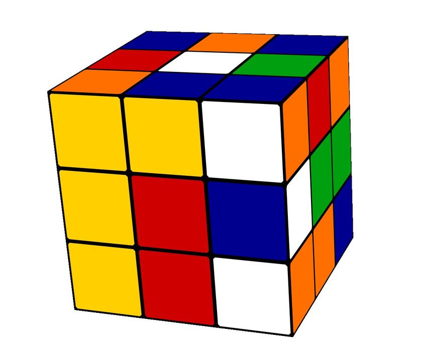
Under review as a conference paper at ICLR 2022

4       E XPERIMENTAL A NALYSIS
For 100 sample cubes, initially randomly shuffled with 1000 moves each, the Kociemba solver
solved with an average solve length of 20.66 moves, while algorithms used by human solvers like
CFOP or Fridrich method take an average of 107.30 moves. DeepCube (McAleer et al., 2018) re-
ported a median solve length of 30 moves over 640 random cubes. Using and evolutionary approach
and incorporating exact methods, El-Sourani et al. (2010) reported an average solve length of 50.31,
with most solves taking 35-45 moves. DeepCubeA (Agostinelli et al., 2019) reported an average
solve length of 21.50 moves, finding the optimal solution 60% of the time, serving as the state of
the art for learning based solvers. The solve lengths and some statistics of the different methods are
summarised in Table 1.

                                               Method                             Solve Length (moves)                                  Time per solve                 Number of Solves
                Beginner                                                                     186.07                                          0.1 sec                              100 / 100
                 CFOP                                                                         107.3                                         0.05 sec                              100 / 100
               Kociemba                                                                       20.66                                         5.291 sec                             100 / 100
               DeepCube∗                                                                       30                                            10 min                               640 / 640
         El-Sourani et al. (2010)∗                                                            50.31                                            N/A                                100 / 100
              DeepCubeA∗                                                                      21.50                                         24.22 sec                               N/A

Table 1: Some statistics to compare different cube solving methods. ∗ - the values are as reported in
the respective publications. While DeepCube has median values, the rest have average values.

CubeTR, at its current version, may not beat these existing solvers in terms of optimality of the
solution. There are cases where the state generation algorithm would explore redundant moves, e.g.
R R R, instead of R’, and the performance could be improved considering these cases. However, the
purpose behind CubeTR was not to obtain an optimal rubik’s cube solver, but actually to explore the
power of transformers in this seemingly disparate2 field of reinforcement learning. Being inspired
by many before it, CubeTR is a simple end-to-end approach with an elegant architectural design.
                                    200
                                               Beginners                                                                                 Beginners
                                    175        CFOP                                                                                      CFOP
                                               Kociemba                                                                         5        Kociemba
                                    150
         Number of moves to solve

                                                                                                                                4
                                                                                                          Time talen to solve

                                    125
                                    100                                                                                         3

                                    75
                                                                                                                                2
                                    50
                                                                                                                                1
                                    25
                                     0                                                                                          0
                                           0         10        20           30          40    50                                    0          10        20           30           40    50
                                                           Number of moves in shuffle                                                                Number of moves in shuffle

                                          (a) Solve Length vs Scramble Length                                                       (b) Time taken vs Scramble Length

5       C ONCLUSION
The transformer is a highly versatile architectural paradigm, that has taken the NLP and CV com-
munities by storm. Though its application in reinforcement learning was proposed recently, this
intersection domain is quite under explored. In the proposed decision transformer, it was shown
that the transformer is able to perform reinforcement learning tasks by reformulating the problem
as a sequence modelling task. CubeTR extends this method by working on the Rubik’s cube, a rep-
resentationally complex combinatorial puzzle that is memoryless and suffers with sparse rewards.
Although all discussions and experiments were conducted with the rubik’s cube in mind, the ar-
chitecture proposed can be applied to other realistic sparse reward scenarios as well. Being the
first work to consider the applications of transformers in solving the rubik’s cube and also the first
one to explore the 4×4 rubik’s cube, CubeTR hopes to serve as a base for future research into the
applications of transformers in the field of reinforcement learning.
    2
        disparate from NLP and CV, where transformers are currently used extensively.

                                                                                                      8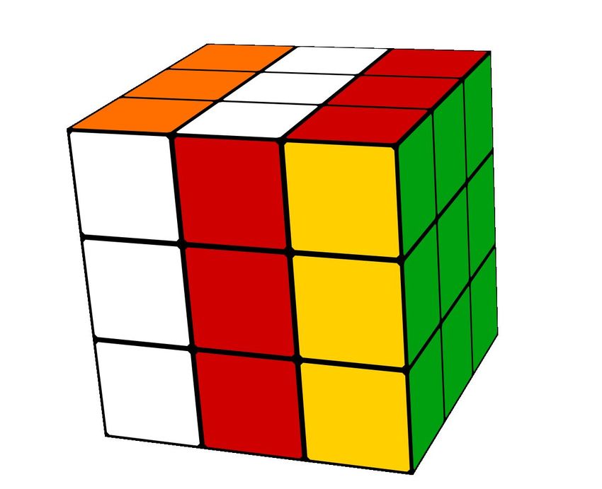
Under review as a conference paper at ICLR 2022

The comparison of CubeTR with other cube solving methods indicate that the approach is far from
optimal. Rather that beating existing methods for solving the rubik’s cube, CubeTR aims to extend
the learning to higher dimensional variants of the cube. The noticable simplicity and intuitive state-
to-action prediction style used was possible primarily because of the great representation power of
transformers. Taking the closer look at the architecture, it may be observed that the basic building
blocks are small variations of off-the-shelf transformer architectures commonly used in CV and
NLP, with very few reinforcement learning specific modifications in the core architecture. This is
clear indication of the versatile nature of the transformer architecture, and supports the exploration
of transformers in other, seemingly disparate, fields of machine learning.

R EFERENCES
Forest Agostinelli, Stephen McAleer, Alexander Shmakov, and Pierre Baldi. Solving the rubik’s
  cube with deep reinforcement learning and search. Nature Machine Intelligence, 1(8):356–363,
  2019.
Najeba Aqra and Najla Abu Salah. Rubik’s cube solver. 2017.
Peter Auer, Nicolo Cesa-Bianchi, and Paul Fischer. Finite-time analysis of the multiarmed bandit
  problem. Machine learning, 47(2):235–256, 2002.
Tom Brown, Benjamin Mann, Nick Ryder, Melanie Subbiah, et al. Language models are few-shot
  learners. In Advances in Neural Information Processing Systems, volume 33, pp. 1877–1901,
  2020.
Robert Brunetto and Otakar Trunda. Deep heuristic-learning in the rubik’s cube domain: An exper-
  imental evaluation. In ITAT, pp. 57–64, 2017.
Yuri Burda, Harri Edwards, Deepak Pathak, Amos Storkey, Trevor Darrell, and Alexei A Efros.
  Large-scale study of curiosity-driven learning. In International Conference on Learning Repre-
  sentations, 2018.
Lili Chen, Kevin Lu, Aravind Rajeswaran, Kimin Lee, Aditya Grover, Michael Laskin, Pieter
  Abbeel, Aravind Srinivas, and Igor Mordatch. Decision transformer: Reinforcement learning
  via sequence modeling. arXiv preprint arXiv:2106.01345, 2021.
Frédéric Dandurand, Denis Cousineau, and Thomas R Shultz. Solving nonogram puzzles by re-
   inforcement learning. In Proceedings of the Annual Meeting of the Cognitive Science Society,
   volume 34, 2012.
Jacob Devlin, Ming-Wei Chang, Kenton Lee, and Kristina Toutanova. Bert: Pre-training of deep
  bidirectional transformers for language understanding. In NAACL-HLT, 2019.
Alexey Dosovitskiy, Lucas Beyer, Alexander Kolesnikov, Dirk Weissenborn, Xiaohua Zhai, Thomas
  Unterthiner, Mostafa Dehghani, Matthias Minderer, Georg Heigold, Sylvain Gelly, et al. An im-
  age is worth 16x16 words: Transformers for image recognition at scale. In International Confer-
  ence on Learning Representations, 2020.
Nail El-Sourani, Sascha Hauke, and Markus Borschbach. An evolutionary approach for solving
  the rubik’s cube incorporating exact methods. In European conference on the applications of
  evolutionary computation, pp. 80–89. Springer, 2010.
Katherine Elkins and Jon Chun. Can gpt-3 pass a writer’s turing test? Journal of Cultural Analytics,
  2020.
Damien Ernst, Mevludin Glavic, Pierre Geurts, and Louis Wehenkel. Approximate value iteration in
  the reinforcement learning context. application to electrical power system control. International
  Journal of Emerging Electric Power Systems, 2005.
Carlos Florensa, David Held, Xinyang Geng, and Pieter Abbeel. Automatic goal generation for
  reinforcement learning agents. In International conference on machine learning, pp. 1515–1528.
  PMLR, 2018.

                                                  9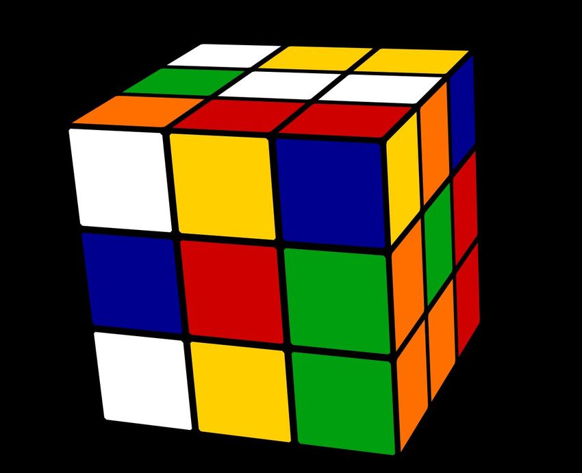
Under review as a conference paper at ICLR 2022

Matthew Hausknecht and Peter Stone. Deep recurrent q-learning for partially observable mdps. In
 2015 aaai fall symposium series, 2015.
Matteo Hessel, Joseph Modayil, Hado Van Hasselt, Tom Schaul, Georg Ostrovski, Will Dabney, Dan
 Horgan, Bilal Piot, Mohammad Azar, and David Silver. Rainbow: Combining improvements in
 deep reinforcement learning. In Thirty-second AAAI conference on artificial intelligence, 2018.
Ziniu Hu, Yuxiao Dong, Kuansan Wang, Kai-Wei Chang, and Yizhou Sun. Gpt-gnn: Generative
  pre-training of graph neural networks. In Proceedings of the 26th ACM SIGKDD International
  Conference on Knowledge Discovery & Data Mining, pp. 1857–1867, 2020.
Kishor Jothimurugan, Osbert Bastani, and Rajeev Alur. Abstract value iteration for hierarchical
  reinforcement learning. In International Conference on Artificial Intelligence and Statistics, pp.
  1162–1170. PMLR, 2021.
John Jumper, Richard Evans, Alexander Pritzel, Tim Green, Michael Figurnov, Olaf Ronneberger,
  Kathryn Tunyasuvunakool, Russ Bates, Augustin Žı́dek, Anna Potapenko, et al. Highly accurate
  protein structure prediction with alphafold. Nature, 2021.
Richard E Korf. A program that learns to solve rubik’s cube. In AAAI, pp. 164–167, 1982.
Daniel Kunkle and Gene Cooperman. Twenty-six moves suffice for rubik’s cube. In Proceedings of
  the 2007 international symposium on Symbolic and algebraic computation, pp. 235–242, 2007.
Keqin Liu and Qing Zhao. Distributed learning in multi-armed bandit with multiple players. IEEE
  Transactions on Signal Processing, 58(11):5667–5681, 2010.
Maja J Mataric. Reward functions for accelerated learning. In Machine learning proceedings 1994,
 pp. 181–189. Elsevier, 1994.
Stephen McAleer, Forest Agostinelli, Alexander Shmakov, and Pierre Baldi. Solving the rubik’s
  cube with approximate policy iteration. In International Conference on Learning Representations,
  2018.
Volodymyr Mnih, Koray Kavukcuoglu, David Silver, Alex Graves, Ioannis Antonoglou, Daan Wier-
  stra, and Martin Riedmiller. Playing atari with deep reinforcement learning. arXiv, 2013.
Volodymyr Mnih, Adria Puigdomenech Badia, Mehdi Mirza, Alex Graves, Timothy Lillicrap, Tim
  Harley, David Silver, and Koray Kavukcuoglu. Asynchronous methods for deep reinforcement
  learning. In International conference on machine learning, pp. 1928–1937. PMLR, 2016.
Seyed Sajad Mousavi, Michael Schukat, and Enda Howley. Deep reinforcement learning: an
  overview. In Proceedings of SAI Intelligent Systems Conference, pp. 426–440. Springer, 2016.
Rémi Munos. Error bounds for approximate value iteration. In Proceedings of the National Confer-
   ence on Artificial Intelligence, volume 20, pp. 1006. Menlo Park, CA; Cambridge, MA; London;
   AAAI Press; MIT Press; 1999, 2005.
Andrew Y Ng, Daishi Harada, and Stuart Russell. Policy invariance under reward transformations:
  Theory and application to reward shaping. In International Conference on Machine Learning,
  1999.
James G Nourse. The Simple Solution to Rubik’s Cube. Bantam, 1981.
Pierre-Yves Oudeyer. Computational theories of curiosity-driven learning.           arXiv preprint
  arXiv:1802.10546, 2018.
Yannis Papanikolaou and Andrea Pierleoni. Dare: Data augmented relation extraction with gpt-2.
  arXiv preprint arXiv:2004.13845, 2020.
Deepak Pathak, Pulkit Agrawal, Alexei A Efros, and Trevor Darrell. Curiosity-driven exploration
  by self-supervised prediction. In International conference on machine learning, pp. 2778–2787.
  PMLR, 2017.

                                                10
Under review as a conference paper at ICLR 2022
Alec Radford, Karthik Narasimhan, Tim Salimans, and Ilya Sutskever. Improving language under-
standing by generative pre-training. 2018.
Alec Radford, Jeffrey Wu, Rewon Child, David Luan, Dario Amodei, Ilya Sutskever, et al. Language
models are unsupervised multitask learners. OpenAI blog, 1(8):9, 2019.
Martin Riedmiller, Roland Hafner, Thomas Lampe, Michael Neunert, Jonas Degrave, Tom Wiele,
Vlad Mnih, Nicolas Heess, and Jost Tobias Springenberg. Learning by playing solving sparse
reward tasks from scratch. In International Conference on Machine Learning, pp. 4344–4353.
PMLR, 2018.
Tomas Rokicki, Herbert Kociemba, Morley Davidson, and John Dethridge. The diameter of the
rubik’s cube group is twenty. siam REVIEW, 56(4):645–670, 2014.
John Schulman, Sergey Levine, Pieter Abbeel, Michael Jordan, and Philipp Moritz. Trust region
policy optimization. In International conference on machine learning, pp. 1889–1897. PMLR,
2015a.
John Schulman, Philipp Moritz, Sergey Levine, Michael Jordan, and Pieter Abbeel. High-
dimensional continuous control using generalized advantage estimation. arXiv preprint
arXiv:1506.02438, 2015b.
David Silver, Aja Huang, Chris J Maddison, Arthur Guez, Laurent Sifre, George Van Den Driessche,
Julian Schrittwieser, Ioannis Antonoglou, Veda Panneershelvam, Marc Lanctot, et al. Mastering
the game of go with deep neural networks and tree search. nature, pp. 484–489, 2016.
David Silver, Thomas Hubert, Julian Schrittwieser, Ioannis Antonoglou, Matthew Lai, Arthur Guez,
Marc Lanctot, Laurent Sifre, Dharshan Kumaran, Thore Graepel, et al. Mastering chess and shogi
by self-play with a general reinforcement learning algorithm. arXiv, 2017.
David Silver, Thomas Hubert, Julian Schrittwieser, Ioannis Antonoglou, Matthew Lai, Arthur Guez,
Marc Lanctot, Laurent Sifre, Dharshan Kumaran, Thore Graepel, et al. A general reinforcement
learning algorithm that masters chess, shogi, and go through self-play. Science, pp. 1140–1144,
2018.
Alexander Trott, Stephan Zheng, Caiming Xiong, and Richard Socher. Keeping your distance:
Solving sparse reward tasks using self-balancing shaped rewards. Advances in Neural Information
Processing Systems, pp. 10376–10386, 2019.
Hado Van Hasselt, Arthur Guez, and David Silver. Deep reinforcement learning with double q-
learning. In Proceedings of the AAAI conference on artificial intelligence, volume 30, 2016.
Ashish Vaswani, Noam Shazeer, Niki Parmar, Jakob Uszkoreit, Llion Jones, Aidan N Gomez,
Łukasz Kaiser, and Illia Polosukhin. Attention is all you need. In Advances in neural information
processing systems, pp. 5998–6008, 2017.
Joannes Vermorel and Mehryar Mohri. Multi-armed bandit algorithms and empirical evaluation. In
European conference on machine learning, pp. 437–448. Springer, 2005.
Sofı́a S Villar, Jack Bowden, and James Wason. Multi-armed bandit models for the optimal design
of clinical trials: benefits and challenges. Statistical science: a review journal of the Institute of
Mathematical Statistics, 30(2):199, 2015.
Yuqing Wang, Zhaoliang Xu, Xinlong Wang, Chunhua Shen, Baoshan Cheng, Hao Shen, and
Huaxia Xia. End-to-end video instance segmentation with transformers. In Proceedings of the
IEEE/CVF Conference on Computer Vision and Pattern Recognition, pp. 8741–8750, 2021.
Ziyu Wang, Tom Schaul, Matteo Hessel, Hado Hasselt, Marc Lanctot, and Nando Freitas. Dueling
network architectures for deep reinforcement learning. In International conference on machine
learning, pp. 1995–2003. PMLR, 2016.
Kenny Young, Gautham Vasan, and Ryan Hayward. Neurohex: A deep q-learning hex agent. In
Computer Games, pp. 3–18. Springer, 2016.
Baochang Zhang, Zhili Mao, Wanquan Liu, and Jianzhuang Liu. Geometric reinforcement learning
for path planning of uavs. Journal of Intelligent & Robotic Systems, 77(2):391–409, 2015.
11You can also read