Detecting Extra-Solar Earths - Shaped Pupil Coronagraphy for NASA's Terrestrial Planet Finder (TPF-C) Mission

Page created by Cecil Ingram
 
CONTINUE READING
Detecting Extra-Solar Earths - Shaped Pupil Coronagraphy for NASA's Terrestrial Planet Finder (TPF-C) Mission
Detecting Extra-Solar Earths
Shaped Pupil Coronagraphy for NASA’s Terrestrial
         Planet Finder (TPF-C) Mission

                    Ruslan Belikov

        Mechanical and Aerospace Engineering Department
                      Princeton University

                                                     Stanford, April 14 2005
Detecting Extra-Solar Earths - Shaped Pupil Coronagraphy for NASA's Terrestrial Planet Finder (TPF-C) Mission
I should disclose and publish to the world the occasion of discovering and observing
four Planets, never seen from the beginning of the world up to our own times,
their positions, and the observations . . . about their movements and their changes
of magnitude; and I summon all astronomers to apply themselves to examine and
determine their periodic times. . . .

— Galileo Galilei, March 1610
Detecting Extra-Solar Earths - Shaped Pupil Coronagraphy for NASA's Terrestrial Planet Finder (TPF-C) Mission
Is Earth Unique?
 •Answer in 2015

 •How common are
 earth-like planets?
 •Do they harbor the
 conditions for life?

“Conduct advanced telescope searches for Earth-like planets and
habitable environments around other stars.”
                                    – A Renewed Spirit of
Discovery: The President’s Vision for Space Exploration, 2004
Detecting Extra-Solar Earths - Shaped Pupil Coronagraphy for NASA's Terrestrial Planet Finder (TPF-C) Mission
Outline

• Background on planet searches and TPF

• The Shaped-Pupil Coronagraph: a solution to
planet imaging

• The challenge: wavefront control
Detecting Extra-Solar Earths - Shaped Pupil Coronagraphy for NASA's Terrestrial Planet Finder (TPF-C) Mission
The Princeton TPF group
Faculty                       Graduate Students
N. Jeremy Kasdin (MAE)        Amir Give’on
Michael Littman (MAE)         Laurent Pueyo
David Spergel (Astro)         Jason Kay
Ed Turner (Astro)
Robert Vanderbei (ORFE)

Staff
Michael Carr (Astro)                         Discover
Ruslan Belikov, Ph.D. (MAE)                  Vol. 23, No. 3
                                             March, 2002
Detecting Extra-Solar Earths - Shaped Pupil Coronagraphy for NASA's Terrestrial Planet Finder (TPF-C) Mission
Are there any planets out there?

There are at least 145
exoplanets known to date!

    This is an “indirect”
    detection method
Detecting Extra-Solar Earths - Shaped Pupil Coronagraphy for NASA's Terrestrial Planet Finder (TPF-C) Mission
Current detection methods

                Astrometric measurements
                of the location of the star
Detecting Extra-Solar Earths - Shaped Pupil Coronagraphy for NASA's Terrestrial Planet Finder (TPF-C) Mission
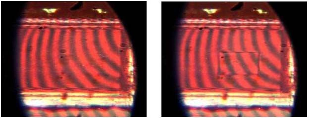
Detected Planets and
Mission Sensitivities

 • Shown are reported
   findings up until
   August 31, 2004.
    – Blue: RV;
    – Red: transits
    – Yellow: microlensing
 • 5-σ limits of different
   techniques shown
 • Need direct imaging to
   detect extra-solar earths
Detecting Extra-Solar Earths - Shaped Pupil Coronagraphy for NASA's Terrestrial Planet Finder (TPF-C) Mission
The only way to find
terrestrial planets is…

Direct detection
Detecting Extra-Solar Earths - Shaped Pupil Coronagraphy for NASA's Terrestrial Planet Finder (TPF-C) Mission
First images of (very large) planets
      2M 1207          •   Left: VLT, IR light with adaptive optics, April
                           2004. Courtesy Gael Chauvin / ESO.
                       •   Right: Hubble, IR light, January 2005.
                           Courtesy NASA / ESA / Glenn H.
                           Schneider, et al
                       •   Brown dwarf host, 8 million years, 1000C, 5
                           Jupiter masses, 54a.u., 2,500 year period

                       •   VLT, NACO adaptive optics infrared
     GQ Lupi               camera, March 2005. Courtesy Ralph
                           Neuhäuser / ESO.
                       •   few million years, 50a.u., 1200 year period,
                           2000K, 1-42 Jupiter masses.

                       •   Spitzer’s IR array camera @ 4.5 and 8
                           microns, October 2004. Courtesy David
                           Charbonneau (Harvard-Smithsonian Center
                           for Astrophysics)
                       •   Spitzer's multiband imaging photometer @
                           24 microns, December 2004. Courtesy
                           Drake Deming (NASA/Goddard Space
                           Flight Center)
The habitable zone

                     The habitable zone,
                     relative to our solar
                     system is defined by the
                     possibility of the
                     existence of liquid water
How hard is this really?
                              •   To minimize glare, image
                                  in the infrared. Problems:
                                   – Much dimmer than visible
                                   – Much worse resolution
                                     than visible

    > 109                     •   NASA’s conclusion: Do a
                                  visible mission first, with
                                  very high contrast
                                  telescope: the TPF-C.
            > 106                  – Photon flux and resolution
                                     acceptable
                                   – 1010 contrast required

              Traub & Jucks
TPF-C

•   2015-2020
•   Detection
     –   35 core nearby stars (150 extended mission)
     –   Distance from star: 0.7-1.5 a.u.
     –   Surface area: 0.5 of Earth and greater
•   Characterization
     –   Orbit, distance
     –   Photometry: size, rotation
     –   Spectroscopy: atmosphere, water
     –   Life
•   General Astrophysics
Photometry
Spectroscopy
Water
Oxygen
Atmospheric Pressure
(Rayleigh Scattering)
Plant Life: Red Edge!

Ref.: Woolf, Smith, Traub, & Jucks, ApJ 2002
Spectra of Plants
Planet Search Mission Schedule

                  Kepler     SIM

                  TPF-C       TPF-I
Outline

• Background on planet searches and TPF

• The Shaped-Pupil Coronagraph: a solution to
planet imaging

• The challenge: wavefront control
Some Existing Coronagraph Types
•Lyot Coronagraphy
   •Attenuates planet light as well
   •Very hard to manufacture
   •Very sensitive to low order aberrations & pointing

•Apodization
  •Difficult to implement
  •Poor accuracy
  •Low Throughput

•Shaped Pupils & Binary Coronagraphs
   •Our favored solution!!
The Problem: Airy rings (sidelobes)
Wavelength (λ)
                                                    Focal plane              The image in the
                                                                             focal plane is the
                                                                             spatial Fourier
                                                                             transform of the
                                                                             entrance field
                                                                    0
                                                               10

                         Diameter (D)                          10 -2

                                                               10 -4

                             FT                                10 -6

                                                                    -8
                                                               10

                                                               10 -10

 Entrance Pupil
                                                               10 -12
                                                                         0       5                      10   15
Size of Image is a function of Telescope Size and Wavelength                         Angle (lambda/D)
The Soluion: Modify Entrance Pupil
Wavelength (λ)
                                                    Focal plane              The image in the
                                                                             focal plane is the
                                                                             spatial Fourier
                                                                             transform of the
                                                                             entrance field
                                                                    0
                                                               10

                         Diameter (D)                          10 -2

                                                               10 -4

                             FT                                10 -6

                                                                    -8
                                                               10

                                                               10 -10

 Entrance Pupil
                                                               10 -12
                                                                         0       5                      10   15
Size of Image is a function of Telescope Size and Wavelength                         Angle (lambda/D)
The optimization problem
Find an apodization function A(r) that solves:

When we wish to consider binary apodizers (i.e. masks), we also add the
constraint that for each opening:

We only consider masks that are symmetric with respect to both the x
and y axes. Hence, the function a() is a nonnegative even function.
Performance metrics
In order to compare the different designs, we use the following metrics:

Size of dark region:
Typically measured using inner and outer working angles: ρiwa and ρowa

Contrast:

Airy throughput:
The energy inside the inner working angle divided by the total energy of
a clear open aperture:
Circular aperture: the Airy pattern

 ρiwa = 1.24
 Tairy = 84.2%

                 No dark zone
Apodization
ρiwa = 4
Tairy = 9%

Excellent dark zone Unmanufacturable
Binary pupil

Excellent dark zone   Impossible to manufacture
1D: Prolate Spheroidal (Slepian, 1963)
                                    Zero-Order Prolate Spheroidal Wave Function                          0
                1                                                                                   10

ρiwa = 4
              0.9                                                                                   10
                                                                                                         -2

              0.8                                                                                        -4
                                                                                                    10

              0.7
                                                                                                         -6
                                                                                                    10

              0.6

Tairy = 25%   0.5
                                                                                                    10
                                                                                                         -8

                                                                                                         -10
                                                                                                    10
              0.4
                                                                                                         -12
                                                                                                    10
              0.3
                                                                                                         -14
                                                                                                    10
              0.2

                                                                                                         -16
              0.1                                                                                   10

                                                                                                         -18
               0                                                                                    10
               -0.5   -0.4   -0.3      -0.2     -0.1       0       0.1      0.2   0.3   0.4   0.5              0   5   10   15

              Analytic solution via
              calculus of variations

    Theoretically optimal for 1-D Unmanufacturable
The Spergel-Kasdin pupil
ρiwa = 4
Tairy = 43%

                                                                                    0
                                                                               10

                                                                                    -2
                                                                               10

                                                                                    -4
                                                                               10

                                                                               10 -6

                                                                               10 -8

                                  Lab image
                                                                                    -10
                                                                               10

                                                                                    -12
                                                                               10

                                                                               10 -14
                            100

                            200
                                                                               10 -16
                            300

                            400
                                                                               10 -18
                            500
                                                                                          0   5   10   15
                            600

                            700

                            800

                            900

                           1000
                                  200   400   600   800   1000   1200   1400

           Optimal across x-axis                                 Very narrow opening
Other designs…
Our favorite…
ρiwa = 4
Tairy = 30%
What would a solar system look like?...

                    Light reflecting off the
                    planet from the star
                                               Star
                                                 Only
                                                    + planet
                                                       star
   Planet
Simulation of a planet
at 20 λ/D with contrast
         −8
of 5*10 relative to the
star
Star light.                                        Telescope

               Planet
                    ~ 30 light years
It really works!!

   31 Leonis is a dim double with magnitudes 4.37/13.6 and
   separation 7.9”
Without Mask                    With Mask

        Courtesy Prof. Robert Vanderbei
Our mask

   Silicon based mask, 200 microns thick (thinned
   to 50 microns near the openings).
It is all fun and games,
until you go to the lab…
                                 Image measured
  Simulated image
                                    in the lab
                    planets???
Our best results to date
   measurement         Horizontal trace through the middle

       simulation

                    Next step: correct aberrations!
Outline

• Background on planet searches and TPF

• The Shaped-Pupil Coronagraph: a solution to
planet imaging

• The challenge: wavefront control
The real challenge:

         Wavefront control
     Phase aberrations       Amplitude aberrations

     Requirement: λ/10,000     Requirement: 1 / 1,000
Simulating the aberration
    Phase aberrations               Amplitude aberrations

 RMS = λ/20                                RMS = 0.01
 (λ = 632nm, given in units of λ)
The resulting image
         The aberrated
           The         image
               ideal image
Deformable mirrors
             Boston Micromachines   Xinetics

Face-sheet

 Actuators
Conventional wavefront
estimation and correction

 Measurements
 are taken at
 the pupil plane

 Cannot correct
 these elements             Diagram by Claire Max, UCSC
Image-plane-based wavefront estimation

    Information is lost - must have diversity!
Image-plane wavefront
estimation techniques:

• Error reduction algorithms (Gerchberg-Saxton)

• Maximum Likelihood techniques

• Optimization-based techniques
Defocus + wavelength diversity
     Challenge: getting diversity without sacrificing valuable photons
                                                    Imaging
                                                    system I

                    Telescope
                                                                         Imaging
                                                                         system II

                                                                Dichroics

                     Shaped                         Imaging
                      pupil                        system III

          The change in wavelength and the defocus provides the
          needed diversity without losing any photons
Correction techniques

• Conventional phase conjugation

• Global optimization techniques

• Fourier coefficients-based correction
Polychromatic amplitude correction

                  Zero-Path
                  Difference
                  Michelson
                  Interferometer
The Challenge:
       Polychromatic amplitude correction
• Phase alone is conceptually easy: use a good DM
• Phase with amplitude is conceptually easy for
  monochromatic light: use 2 interfering DMs.
• Amplitude polychromatically is difficult
• Proposed solution: use a binary chip like the TI DMD
  and dither

                                          ~
Pictures courtesy of Texas Instruments
Putting it all together…
Future work
 • Lab (finally getting deformable mirrors!!)

 • Mask designs

 • Mask manufacturing

 • Estimation techniques

 • Correction techniques
Conclusions
• An imaging telescope in the visible is the best approach
for earth-like planet detection, but requires 1010 contrast.
• The Princeton TPF team has designed the Shaped Pupil
Coronagraph as a solution to the high contrast problem
• The main challenge is wavefront control. The TPF group
at Princeton is developing methods, algorithms, and
significant laboratory capability to correct the wavefront
to the required levels
•Within 10 years, we will see the first extrasolar terrestrial
planet!
Thank you
You can also read