Development of simulator for Schunk Powerball Arm

1. Development of simulator for Schunk Powerball Arm
1.1 Introduction

Computerized simulations play a vital role in understanding the motion of devices like robotic
arms. They are widely used to predict the motion of the arm and detect any flaws in the
proposed motion. Thus they play an important role in preventing damage. Besides this,
simulations are widely used in motion planning during the learning phase of the bot. Keeping
these uses in mind, the project aimed to develop a model as accurate as possible for the
Schunk Powerball arm. As a part of the project, two simulations were created, one in a
commercial software and the other one in the indigenous software being developed at the
lab called the RPI Matlab simulator.

1.2 Commercial software simulation

Solidworks 2012 was chosen for the
purpose of developing the simulation as it
was easily accessible and widely used in
the student community. The Powerball
was divided into seven parts which were
assembled sequentially. Solidworks allows
control of position as well as joint torques
for simulations. A dummy hand was
placed on the arm. It resulted in a total of
six motors placed in the simulation. A
separate gripper was also simulated in the
software. This model could perform the
basic functions of the arm. For the
Powerball to follow any specific trajectory,
the trajectory angles can be input into the
simulation in .csv format. The simulation
also offers calculation of joint torques and
forces at various positions in the arm. An
example for the same has been attached
in appendix A

The main challenge in developing the simulation in Solidworks was making accurate models
of the Powerball arm due to severe lack of documentation in this aspect from Schunk.

Although the simulation performed as expected in a few basic tests, actual performance
could not be verified because at the time of this report, the real Powerball was not functional.

1.3 Simulation on Matlab Simulator

The main purpose of developing the simulation on the Matlab simulator was to compare the
results obtained from the commercial software with those from the simulator. The simulator
also performs quite well on certain other aspects like collision detection. Currently most of
the algorithms used for collision detection are not accurate. They generate forces after a

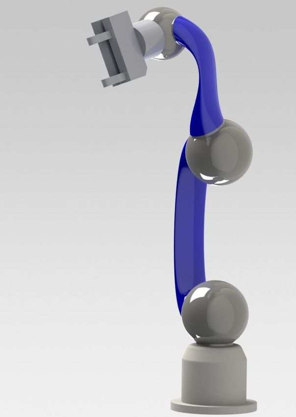
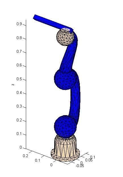
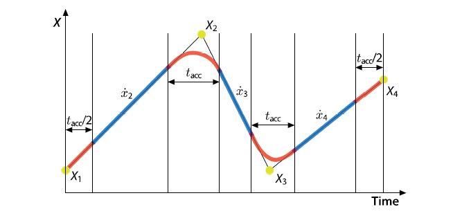
certain level of penetration has been achieved whereas the current simulator is much more
accurate (which will be discussed later).

1.3.1 Kinematic model

The geometric and physical models
developed in Solidworks were imported
into the Matlab simulator using Blender.
The first task was to develop a kinematic
model of the arm. The model was setup
such that initially it is in zero position as
shown in the figure.

Thus the simulation is ended at zero time
steps and the final pose is calculated for
the arm. An example for the final pose of
[0,0,0,0,0,0,0] angle can be seen as in
figure. Please refer appendix B for a
labelled figure of joints

1.3.2 Generation of trajectory motion

The next step was to make the arm follow a particular trajectory to reach the final position.
For generation of trajectories, Peter Corkes Maltab Toolbox was used. The trajectories were
setup follow a continuous path with no sudden jerks. The formulation used for generating
trajectories is:

The motion is completed such that each joint angle is changed gradually to its final position.
We can follow a particular trajectory by introducing intermediary steps between the initial and
final positions. A sample with two intermediary points can be shown as:

Here, we specify the tacc we require which can depend on the maximum acceleration which
can be provided by the actuators.

1.3.3 Dynamic Simulation without collision avoidance

The next step in the simulation was to develop a dynamics simulation for the arm. A PD
controller was used for this purpose with the constants Ka and Kp being 5 and 1
respectively. It was setup such that for any final Joint angle configuration [a1, a2, a3, a4, a5,
a6], the final position is reached in a total of 400 time steps. The total angel movement is
divided into 400 time steps such that at each time step, the desired angel is

                         Theta = (Time Step*(Theta Desired))/400

Thus a joint torque proportional to this is applied to the bodies. An equal and opposite torque
is also applied to the preceding body to simulate the forces applied by a motor.

The typical time profile for the simulation can be shown by: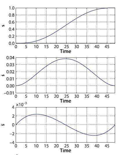

1.3.4 Dynamic Simulation with Collision detection

The next step was to introduce collision avoidance in the model so that the arm can interact
with its environment. As discussed in above, most of the commercially used collision
detection algorithms are not very accurate. In the simulator, a formulation provided by
Stewart Trinkle is already implemented. It has the formulation

                           0  ( z)  z  0

Where z represents the force between any two potential contact vertices and F is a function
of z which represents the distance between the vertices, which can derived from Newtonian
mechanics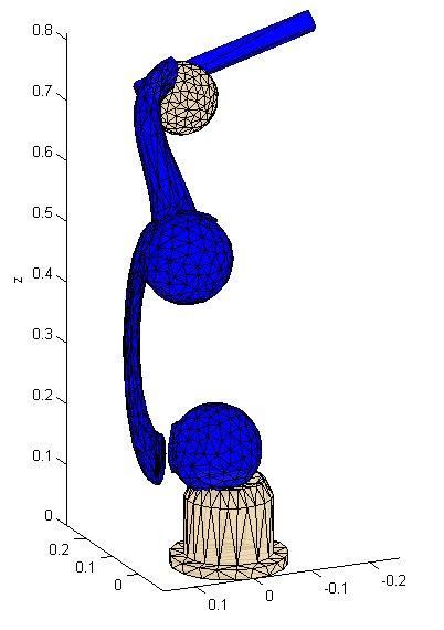

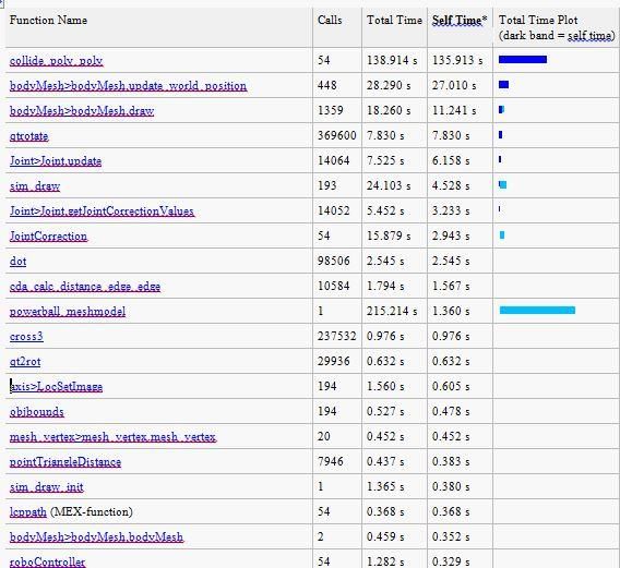
But on introducing collision avoidance in the simulation, we found that the simulation slowed
excessively. A typical time profile for a simulation can be presented as

Thus we see that collision detection (collide_poly_poly) takes most of the time. Even though
in the above simulation, only two objects with simple geometries were being checked for
collisions, but as the algorithm checks every vertex of one body for possible collision, it is
very time consuming. For resolving the time required for the collision detection, BULLET
physics can be used which can produce fairly accurate results at high speeds. We could not
do the BULLET collision detection as BULLET libraries can only be used in 32 bit Ubuntu,
not 64 bit Ubuntu and by the time we realised it, there was not enough time. The next big
thing is the draw functions (update_world_positions) in the Matlab window. We solved the
latter problem by disabling the gui and recording it rather than displaying it directly.

Solving LCP did not take much long (lcppath) as is evident by its placement near the bottom
of the list which is sorted out by time elapsed during that function (the top 20 functions in the
sorting order are shown above).

On comparing the profiles for simulations without collision detection and with collision
detection, we find that the main time consuming operations were Joint update (Joint.update)

and draw functions (update_world_positions). With collision detection dominates the time
profile. Another thing to watch out is that the Join.update function takes more time without
collisions and lesser time with collisions. It can be attributed to the fact that without collisions,
it ran more number of steps and it had to iterate more for the joints(an issue covered in the
next section) whereas when it ran lesser number of step, the joint iterations did not take
much time and drawing took more time,

Another issue which cropped up during simulations was the accumulation of errors in the
joint positions. An example for the same can be illustrated as:

                               Arm falling apart as joint errors accumulate

1.3.5 Maximal and Minimal Coordinate Formulations

As the current formulation uses the maximal coordinate system, a possible solution can be
the use of minimal coordinate technique for joint pose calculation. The maximal coordinate
system uses the penalty force method which can handle both holonomic as well as non
holonomic constraints. It works by creating implicit functions C = 0. After every time step, if
the constraint is satisfied, then it does nothing but if the constraint is not satisfied, it applies a
force to bodies involved in the constraint to fulfil the constraint. For joints used in the
Powerball arm, it is carried out in two steps, in the first step, the position is corrected and
then in the second one, the velocities are corrected. This is iterated over and over until the
error is reduced to a certain value. This method produces very good results if the number of
bodies is relatively small in number. But as the number of bodies increase, the number of
iterations required for constrains to be satisfied increases and so does the small numerical
errors in the formulation which eventually add up to a large number. Because the constraints
will be satisfied sequentially, satisfying one will apply a force which will violate the previous
constraint thus making it very difficult to satisfy all accurately.

Whereas the minimal coordinate system integrates the constraints in the Jacobian for the
applied forces which makes it possible to calculate the positions correctly in the first iteration.
But the problem which is commonly faced with making minimal coordinate formulation is the
formation of Jacobian matrices which satisfy the given constraints.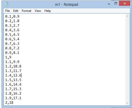

Future Work and Conclusion

The current capability of the simulation is limited to pushing objects which do not require
large changes in angles. But by implementing BULLET collision detection and minimal
coordinate formulation (or by diagnosing the implemented maximal coordinate formulation),
we can achieve better results from the simulation.

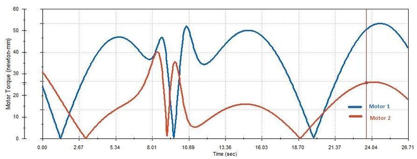
Appendix A

1. Csv file

Each motor in the assembly has to be provided with a separate csv file. An example of a csv
file opened with text editor is:

The first column represents the time (in secs) and the second column may represent any
one of position/velocity/torque for the motors. In this example, position was used.

The resultant Torques required for motors at joint 1 and 2 when the joints are moving at a
constant angular velocity given by [9,9,6,5,4,3] deg/sec for each joint repectively can be
shown as:

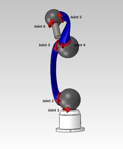
Appendix B

The Joint Angle set labelled as [a1,a2,a3,a4,a5,a6] refer to [J(1), J(2), J(3), J(4), J(5), J(6)]
where J(i) represents Joint  .