Doppler-Free Saturation Spectroscopy - Thomas Rieger and Thomas Volz
←
→
Page content transcription
If your browser does not render page correctly, please read the page content below
Doppler-Free Saturation
    Spectroscopy

     Thomas Rieger and Thomas Volz
 Max-Planck-Institut für Quantenoptik, Garching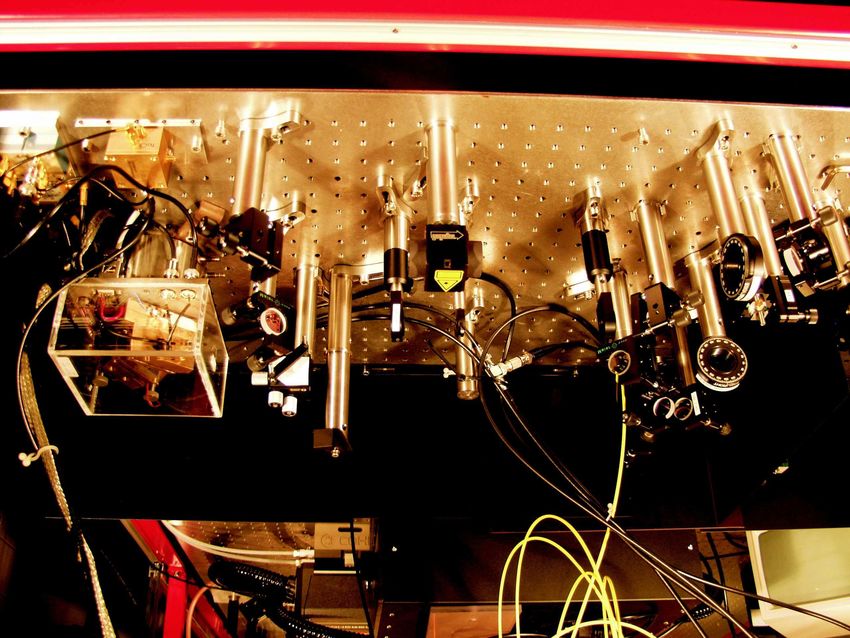
1     Introduction
With the advent of the laser in the 1960s, precision spectroscopy of atoms
and molecules became possible. The laser, being a very narrow, tunable
and coherent light source, allowed to resolve features in atomic and molec-
ular spectra with an unprecedented resolution and accuracy, which led to
a better understanding of the structure of atoms and molecules. Precision
spectroscopy became a very active field and within a short time, a wide
range of different spectroscopic techniques were developed. A good review
is for instance the article [1] written by T. W. Hänsch, A. L. Schawlow and
G. W. Series, which gives an overview of precision spectroscopy of atomic
hydrogen. Many of the basic principles and techniques can be understood
from this article and are still not outdated. Another very good and com-
prehensive introduction on a more detailed basis is given in the book ”Laser
Spectroscopy” by W. Demtröder [2], one of the pioneers of the field.
Laser spectroscopy also paved the way towards all the exciting developments
that took place in the past two decades in the field of laser cooling and trap-
ping of atoms which culminated in 1995 with the realisation of Bose-Einstein
condensation in alkali gases [3]. In all the labs dealing with laser cooling
and trapping of atoms, the technique of Doppler-free saturated absorption
spectroscopy is frequently used as a tool for locking the lasers to particu-
lar atomic lines. In this graduate-student lab experiment, this technique is
introduced in theory and experiment.

2     Saturation Spectroscopy
2.1    Qualitative Picture for Two-Level Atoms
The experimental setup for doing Doppler-free saturation spectroscopy is
shown in Fig. 1. Two counter-propagating laser beams derived from a single
laser beam are sent through an atomic vapour cell. While the ”pump” beam
has a high intensity and serves to bleach the atomic gas, i.e. to make the
gas transparent, the transmittance of the ”probe” beam through the atomic
vapour is recorded with a photodiode and gives the actual spectroscopic sig-
nal. Typically the probe beam has a factor of ten smaller intensity.
In order to understand what kind of signals one can expect, let us for sim-
plicity consider (fictitious) atoms with only two internal states, the ground

                                      1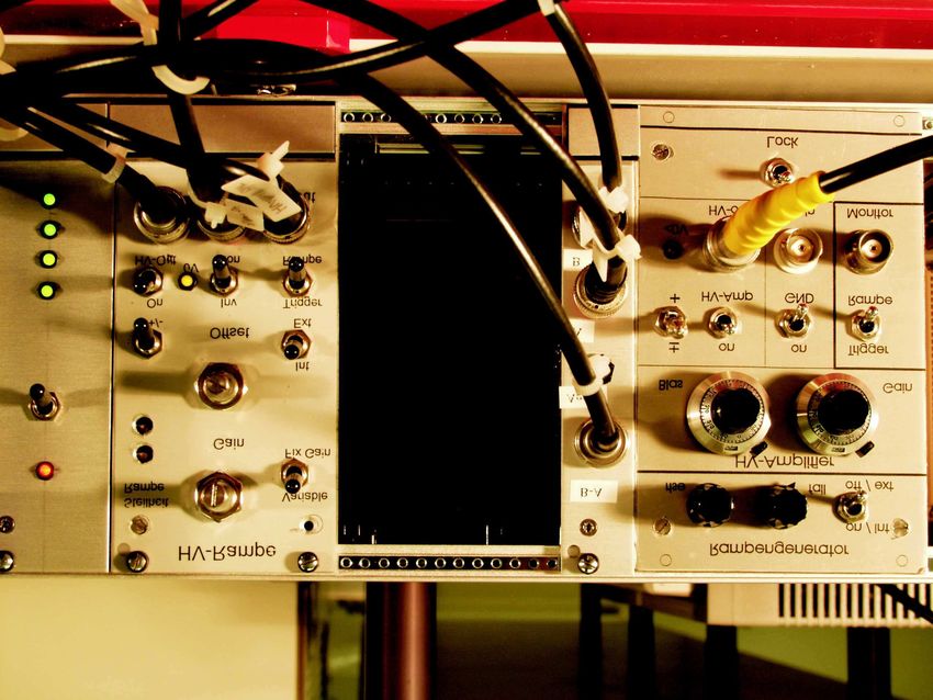
photo diode

             probe                                    pump
             beam              vapour cell            beam

  Figure 1: Basic experimental arrangement for saturation spectroscopy.

state |gi and the excited state |ei. Then, the kind of signals one would get
when scanning the laser frequency are shown in Fig. 2. If the pump beam
is blocked and only the probe beam goes through the vapour cell, one ob-
tains a simple absorption line exhibiting a strong Doppler broadening. Note
the typical Gaussian absorption profile. Typically, the Doppler broadening
at room temperature exceeds the natural linewidth, that is the intrinsic fre-
quency width of an atomic transition, by two orders of magnitude.
Problem 1 Derive a formula for the Doppler-broadening of atomic transi-
tions in terms of the resonance frequency ν0 , the temperature T and atomic
mass m. What is the Doppler broadening for the D-lines in rubidium (ν0 ≈
3.84 · 1014 Hz) at room temperature? The natural linewidth of the transition
is Γ ≈ 6Mhz.
Now, if in addition the pump beam is sent through the vapour cell, a very
narrow spike appears in the probe-beam signal at the resonance frequency
ν = ν0 of the atomic transition. This is the so-called Lamb dip, named after
W. Lamb who first recognized the huge potential of saturation spectroscopy.
   The reason for this spike to show up is the following: only for atoms
having zero velocity along the long axis of the vapour cell the two counter-
propagating laser beams have the same frequency. Atoms moving e.g. to the
right see the frequency of the pump beam shifted into the blue whereas for
the same atoms the probe beam is red-shifted. Hence, whenever atoms with
v 6= 0 see the probe beam shifted into resonance due to the Doppler effect,
at the same time the pump beam is shifted further away from resonance.
    Atoms at zero velocity, however, do see both the pump and the probe
beam. The high intensity or equivalently the high photon flux in the pump
beam, leads to a high absorption rate. The atoms absorb photons from
the pump beam and undergo a transition to the excited state, from where

                                     2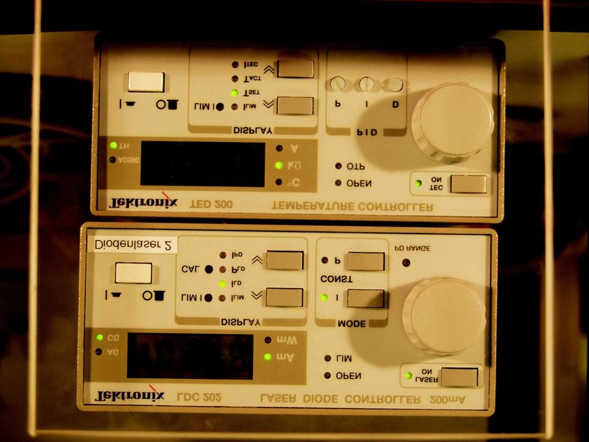
1,0

                                         0,8

                    Probe Transmission
                                         0,6

                                         0,4

                                         0,2

                                         0,0
                                                -500        0         500

                                               detuning from resonance (MHz)

                                         1,0

                                         0,8
                    Probe Transmission

                                         0,6

                                         0,4

                                         0,2

                                         0,0
                                                -500        0         500

                                               detuning from resonance (MHz)

Figure 2: Transmission signal for a probe beam without (a) and with (b) an
intense pump beam present.

they eventually fall back to the ground state by spontaneous emission. If
the pump-beam intensity is high enough, the ground state is significantly
depleted and therefore the absorbance of the probe beam is reduced com-
pared to the case without pump beam: a spike appears in the transmission
spectrum of the probe beam. Note, that for infinite intensity of the pump
beam, on average half of the atoms would be in the excited state and no
probe absorption would occur (next section). This is called ”saturation” of
the atomic transition. Hence, the name ”saturation spectroscopy”.
    The last remark of this section concerns the width of the Lamb dip.
Obviously the dip is much narrower than the Doppler width. If the intrin-
sic frequency width (linewidth) of the laser used in the experiment is small

                                                           3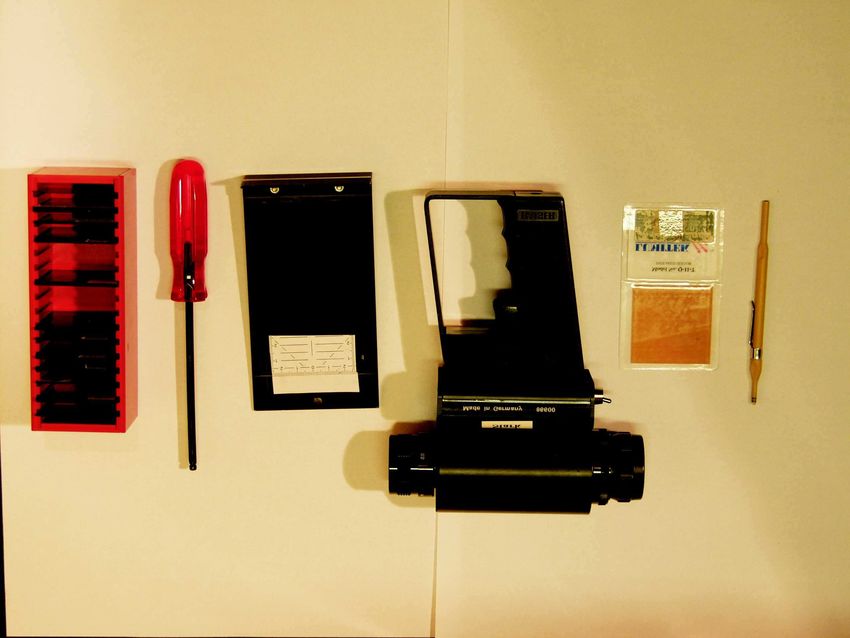
enough, the observed width of the Lamb dip can be as small as the natural
linewidth of the atomic transition.

2.2    Quantitative Picture for Two-Level Atoms
It is fairly straightforward to calculate a crude saturated-absorption spectrum
for a two-level atom. A lot of the underlying physics can be understood from
such a model.

Optical Depth
The intensity I of a single weak laser beam propagating through a vapour
cell changes according to Beer’s law as

                              dI/dx = −αI ,                                 (1)

where α = α(ν) is the frequency-dependent extinction coefficient. In the
case of a single weak beam, to a good approximation α does not depend on
position. Then, the overall transmission through the vapour cell of length l
is given by

                       Iout = Iin e−α(ν)l = Iin e−τ (ν) ,                   (2)

where τ (ν) = α(ν)l is called the optical depth. The contribution from one
velocity class of atoms (v, v + dv) to τ (ν) can be written as

                         dτ (ν, v) = lσ(ν, v)dn(v) .                        (3)

The absorption coefficient σ(ν, v) has a Lorentzian profile with natural linewidth
Γ and a Doppler-shifted resonance frequency
                                        Γ2 /4
                 σ(ν, v) = σ0                            .                  (4)
                              (ν − ν0 + ν0 v/c)2 + Γ2 /4
σ0 is the on-resonance absorption cross section. In general, it depends on
the character of the atomic transition (dipole, quadrupole, etc.) and the
polarization of the incident light (see e.g. Ref.[4]).
The fraction of atoms dn(v) belonging to a certain velocity class follows a
Boltzmann distribution
                                s
                                      m        2
                   dn(v) = n0              e−mv /2kB T dv .                 (5)
                                    2πkB T

                                          4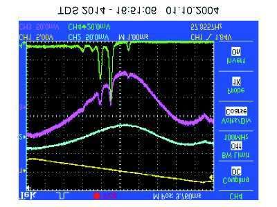
with n0 = N/V being the density of atoms in the vapour cell. Putting
everything together, we obtain the differential contribution to the optical
depth for laser frequency ν and atomic velocity v
                              2 τ0 ν0             2
                dτ (ν, v) =            σ(ν, v)e−mv /2kB T dv ,              (6)
                              π σ0 Γ c
where the overall normalization
                    R
                                  is chosen such that τ0 is the optical depth at
resonance, i.e. τ0 = dτ (ν0 , v) with the integral over all velocity classes.
Problem 2: Under the assumption that the natural linewidth of the atomic
transition is much smaller than the Doppler width, i.e. Γ ¿ ∆D , derive an
expression for the on-resonance optical depth τ0 in terms of σ0 ,n0 , Γ and ∆D .
Discuss your result.

For the situation of Doppler-free saturation spectroscopy we need to account
for the effect of the additional strong pump beam. Due to the presence of this
strong laser beam a significant part of the atoms in the vapour cell will be in
their excited state. And since atoms can only absorb light when they are in
the ground state, we need to insert a factor NgN−Ne
                                                    in the above formula (6),
describing the difference between excited state population Ne and ground
state population Ng .
Rate Equations
The populations in the two states follow the rate equations

                         Ṅg =  ΓNe − σΦ(Ng − Ne )                          (7)
                         Ṅe = −ΓNe + σΦ(Ng − Ne ) ,                        (8)

where the first term in each equation stems from spontaneous emission and
the second term from stimulated processes. Φ = I/hν is the incident photon
flux. Next, Ng can be eliminated using Ng + Ne = N = const. Then, all the
physics is contained in the equation for Ne

                       Ṅe = − (ΓNe + 2σΦ) Ne + σΦN .                       (9)

This differential equation is solved by
                   ·                      ¸
                              N σΦ                 N σΦ
          Ne (t) = ΓNe (0) −         e−(Γ+2σΦ)t +         .                (10)
                             Γ + 2σΦ              Γ + 2σΦ
Several examples of this general solution are shown in Fig. 3: In the case of

                                         5
(a) 1,0
(b) 1,0
0,8 0,8
/ N
0,6
/ N
0,6
5 5
e
e
N
0,4
1 0,4
N
1
0,2 0,2
0,0 0,0
0,0 0,5 1,0 1,5 2,0 0,0 0,5 1,0 1,5 2,0
t t
Figure 3: Excited-state population Ne as a function of time. Fig. (a) shows
an exponential decay of population with Ne (t = 0) = N , in Fig. (b) the
population in Ne increases exponentially in time. In any case the population
in the excited state satisfies Ne < N/2 for long times.
no radiation field present, the system exhibits a purely exponential decay
Ne (t) = Ne (0)e−Γt . (11)
With a weak light source present, i.e. σΦ ¿ Γ, and with initially all pop-
ulation in the ground state, the population in the excited state increases
as
N σΦ h i
Ne (t) = 1 − e−Γt , (12)
Γ
and after a time Γ−1 reaches a very small steady-state population N σΦ/Γ ¿
N . However, in the experiment, we are dealing with a very strong pump
laser. For σΦ À Γ, we get a fully saturated transition
Ne (t) = [Ne (0) − N/2] e−2σΦt + N/2 → N/2 . (13)
Here, saturation means, that half the population is in the excited state. Even
for infinite power, it is therefore not possible to have more than half of the
atoms in the excited state - at least for a two-level system. Lasers rely on
population inversion and therefore involve at least three atomic levels.
6Another effect well-known in laser spectroscopy is power broadening, which
is also present in the steady-state solutions of Eqn.(10). In the limit (Γ +
2σΦ)t À 1, we get
Ne (∞) σΦ
= . (14)
N Γ + 2σΦ
Using expression Eqn. (4) and writing ∆ν = (ν − ν0 − ν0 v/c) (note the minus
sign, due to the opposite Doppler shift for the pump beam compared to the
probe beam), we can rearrange that expression and obtain
Ne (∞) σ0 ΦΓ/4
= . (15)
N ∆ν 2 + Γ2 /4 + σ0 ΦΓ/2
This is a Lorentzian whose ”power-broadened” half width now depends on
the incident photon flux
µ ¶1/2
2σ0 Φ
∆1/2 = Γ/2 1 + . (16)
Γ
Introducing the saturation parameter s = Φ/Φsat , where Φsat = Γ/2σ0 , we
obtain a very convenient formula for the population in the excited state
s/2
Ne = . (17)
1 + s + 4∆2 /Γ2
With this expression for the excited-state population Ne in terms of detuning
∆ and saturation parameter s, we have all the ingredients we need to calculate
a simple saturated-absorption spectrum for a two-level atom.
Let us conclude this section by noting that the saturation intensity Isat can
be expressed as [4]
Isat = 2π 2 hcΓ/3λ3 . (18)
For the D2 line in 87 Rb with a natural linewidth of Γ = 6 MHz, the satura-
tion intensity is Isat ≈ 1.65 mW/cm2 .
Calculated Saturated-Absorption Spectra
In the last two paragraphs we have seen, that a saturated absorption spec-
trum is basically determined by two externally adjustable parameters, namely
the pump intensity and the on-resonance optical depth. Assuming a fixed
7(a) 1,0
Probe Transmission
0,8
0,6
0,4
0,2
0,0
-1000 -500 0 500 1000
detuning from resonance (MHz)
(b) 1,0
Probe Transmission
0,8
0,6
0,4
0,2
0,0
-200 -100 0 100 200
detuning from resonance (MHz)
Figure 4: Probe transmission as a function of laser frequency for different
vapour densities. Fig. (b) is a zoom into the region around ν0 : for very high
densities the saturated-absorption peak vanishes.
temperature and choosing a particular atomic species the latter is propor-
tional to the vapour density inside the cell (also see Problem 1). Fig. 4
shows absorption spectra for different densities in the cell. At low densities,
the probe absorption is weak and shows a Gaussian profile. When increas-
ing the density, the absorption increases and the profile gets broader and
deeper. For even higher densities, the depth is saturated but the width fur-
ther increases, the profile looses its Gaussian shape. The density of absorbing
atoms is so high, that even far from resonance the probe gets absorbed almost
completely. On resonance the absorption is reduced due to the effect of the
strong pump beam and we recognize the saturated absorption feature. For
increasing density, however, this feature becomes smaller and smaller (com-
8pare Fig. 4b). Increasing the atomic density and holding the pump beam
intensity fixed, corresponds to an increase in the absolute number of atoms
in the ground state: the absorption at ν = ν0 increases. In Fig. 5 the density
1,0
Probe Transmission
0,8
0,6
0,4
-100 0 100
detuning from resonance (MHz)
Figure 5: Saturated-absorption peak at ν = ν0 for fixed vapour density
and varying pump beam intensity. The effect of power broadening is clearly
visible.
is fixed and the intensity of the pump beam is varied. For higher intensities,
the Lamb dip becomes higher and broader: the pump beam saturates and
power-broadens the atomic transition.
3 Multilevel Atoms - Alkalis
Alkali atoms are the workhorse in many of today’s experiments dealing with
the trapping, cooling and manipulation of atoms. Their popularity has mul-
tiple reasons. Most important is their relatively simple hydrogen-like level
structure due to a single valence electron in the outer shell. In contrast to hy-
drogen, however, the transition frequency from the ground to the first excited
state typically lies in the visible or near-infrared part of the spectrum, which
can be conveniently accessed by relatively cheap and reliable lasers that are
commercially available. In this experiment, for example, rubidium is used
with a transition frequency at 780 nm, for which light can be generated by
standard diode lasers (see for example Refs. [4, 5]).
93.1 Fine-Structure Splitting
In the case of rubidium the inner four electronic shells are filled, and only the
single outer (5s) valence electron determines the angular momentum config-
uration of the atom. The state of the electron is completely described by its
orbital angular momentum L ~ and its spin S.~ These two angular momenta
couple in the usual way to form the total angular momentum J of the elec-
tron. Hence, J can take the values |L − S| ≤ J ≤ |L + S|. Responsible for
the coupling is the so-called spin-orbit interaction, which can be written as
~ · S.
Vso = Af s L ~ It is a relativistic effect and can be readily derived from
the Dirac equation for spin-1/2 particles. Simply speaking, the spin-orbit
coupling is nothing else but the magnetic interaction energy of the electronic
spin in the magnetic field due to the relative motion of nucleus and electron.
For details, see any good book on (relativistic) quantum mechanics. The
spin-orbit coupling leads to the so-called fine-structure splitting for different
values of the total angular momentum J. ~
For the alkali atoms the electronic states are fully specified in the so-called
Russell-Saunders notation n(2S+1) LJ , where n denotes the principal electronic
quantum number. Hence, n = 5 in the case of Rb, and its ground state is
given by 52 S1/2 . The fine-structure splitting between the first excited states
52 P1/2 and 52 P3/2 is 7123 GHz.
3.2 Hyperfine-Structure Splitting
If the rubidium nucleus carried no spin, the 52 S1/2 , 52 P1/2 and 52 P3/2 energy
levels would be singlets with no external fields applied. However, this is not
true; there are two natural isotopes of rubidium: 87 Rb with a nuclear spin
of I = 3/2 and 85 Rb with I = 5/2 and a higher abundance level of 72%.
The non-vanishing nuclear spins have magnetic and (electric) quadrupolar
moments associated with them, leading to the so-called hyperfine splitting
of the atomic energy levels.
The first contribution to the hyperfine splitting is the energy of the nuclear
magnetic (dipole) moment ~µnucl in the magnetic field B ~ el generated by the
valence electron at the position of the nucleus
hf
Hmagn ~ el .
= −~µnucl · B (19)
Since ~µnucl is proportional to the nuclear spin I~ and B
~ el is proportional to the
total angular momentum of the valence electron J, ~ H hf can be rewritten as
magn
10αI~ · J.
~ The parameter α is called the magnetic hyperfine structure constant
and has units of energy, that is I~ and J~ are taken to be dimensionless.
A second contribution to the hyperfine splitting arises from the electro-
static interaction between the valence electron and the non-vanishing electric
quadrupole moment of the nucleus. This interaction can be reexpressed in
terms of the nuclear and electron angular momenta I~ and J~ as follows [3]
β ~ 2 + 3 (I~J)
hf
Hquadr = [3(I~J) ~ − I(I + 1)J(J + 1)], (20)
2I(2I − 1)J(2J − 1) 2
where -in analogy to the magnetic case- β is called the electric quadrupole
interaction constant and has units of energy.
These two interactions lead to a coupling of the nuclear angular momentum
I~ and the electron angular momentum J~ to the total angular momentum
F~ = I~ + J,
~ where F can take any value between |J − I| and J + I. Associated
with the coupling is a splitting into hyperfine levels, which are labelled by the
hyperfine quantum number F. Electric dipole transitions between hyperfine
levels must obey the selection rules
∆L = ±1 (21)
∆F = 0, ±1 (not 0 → 0). (22)
∆J = 0, ±1 (23)
Using the definition for F~ and forming F~ · F~ , it is possible to write I~ · J~ =
[F (F + 1) − J(J + 1) − I(I + 1)]/2 =: C/2. Hence, for given J and I, the
frequencies νF of the various hyperfine levels are given by
AC 3C(C + 1) − 4I(I + 1)J(J + 1)
νF = νJ + + B[ ], (24)
2 8I(2I − 1)J(2J − 1)
where νJ is the frequency (energy) of the state n(2S+1) LJ without the hyper-
fine interaction. In the above expression A = α/h̄ and B = β/h̄ have units
of Hz.
3.3 Rubidium Level Scheme
It turns out that for the 52 S1/2 ground state of both 85
Rb and 87
Rb, the last
term in
11F=3 F=4
121 MHz
267 MHz
5P3/2 F=3
63 MHz
F=2 F=2
29 MHz F=1
157 MHz
F=1
72 MHz
F=0
780.24 nm 780.24 nm
F=2
F=3
5S1/2 6.835 GHz 3.0365 GHz
F=2
F=1
87 85
Rb Rb
85 87
Figure 6: Level scheme for the 5S1/2 → 5P3/2 transition in Rb and Rb.
12Eq.(24) is zero, and thus the hyperfine splitting in the ground state is
characterized by a single parameter A(52 S1/2 ), which for 87 Rb is A(52 S1/2 ) =
3417.34 MHz and for 85 Rb A(52 S1/2 ) = 1011.91 MHz. In contrast, for the
first excited states 52 P1/2 and 52 P3/2 the hyperfine parameters A and B are
both different from zero and typically on the order of a few tens of MHz, i.e.
much smaller than for the ground state. Energy level diagrams of the states
52 S1/2 , 52 P1/2 and 52 P3/2 for both 85 Rb and 87 Rb are shown in Fig. 6. Exact
values for A and B can be found in the literature (Ref.[3]).
It is the main goal of this experiment to measure the hyperfine
constants (A,B) for the state 52 P3/2 of the two isotopes of rubidium.
4 Experiment
4.1 Equipment and Layout
Laser
In the experiment, a home-built external cavity diode laser is used as a light
source. The laser head contains a 780nm high-power AlGaAs semiconduc-
tor laser diode from Sharp (LTD025MD0) together with a collimating lens,
mounted on a temperature-controlled stage. In addition, a diffraction grating
provides feedback by acting as a wavelength selective mirror. The grating
forms one end of the laser cavity and allows fine tuning of the laser’s output
frequency: the grating is mounted on a piezo which can be controlled by ap-
plying a high voltage. Besides, a change in diode temperature and/or diode
current will also drastically(!) affect the output frequency (and power) of
the laser. Hence, unless told otherwise, we strongly recommend not to touch
the laser’s current/temperature control unit (see Fig. 8). For more details
on external cavity diode lasers see for instance Ref. [5].
Fig. 9 shows a photograph of an electronics rack containing two high-
voltage boards (”HV-Rampe” and ”Rampengenerator”) and one small board
with a summing amplifier circuit (”Adder”). With the ”HV-Rampe” the
laser’s output frequency can be scanned. The three knobs of interest control
the voltage ramp that is applied to the grating-piezo: the ”Gain” knob deter-
mines the amplitude of the sweep, with the ”Offset” knob the overall voltage
offset can be adjusted and the ramp speed of the forward and backward
ramps are controlled by the two potentiometers ”Steilheit Rampe”. With
the ”Int/Ext” switch, the voltage ramp can be completely switched off. The
13to
wavemeter fiber coupler
anamorphic
prisms
diode
laser l/4
to experiment
l/2 pol. beam
cube
faraday isolator
anamorphic
diode prisms
to wavemeter
laser
telescope
to exp.
faraday
isolator
Figure 7: Home-built external cavity diode laser and some additional optics.
Do not touch this part of the experiment. Miss-alignment can cause several
hours of time delay!
14Figure 8: Current and temperature controller for diode laser. Settings should
not be changed.
”HV-Rampe” has two outputs, one delivering the high-voltage for the piezo,
the other giving a TTL-level signal (0/+5V) which can be used to trigger
the oscilloscope used for data acquisition. The switch ”Trigger/Rampe” se-
lects between a square pulse and a ramp. Note, that the high-voltage board
”Rampengenerator” has exactly the same features.
Fabry-Perot Interferometer
The aim of this experiment is the determination of hyperfine constants (A,B).
In order to extract quantitatively the energy splitting of the different hyper-
fine levels from measured spectra, a reference frequency is needed for cal-
ibration. Here, the Fabry-Perot interferometer comes into play. Such an
interferometer consists of two highly-reflecting mirrors forming an optical
cavity. For a given distance L between the mirrors, light is only transmit-
ted through the cavity, if a standing wave can build up between the two
mirrors, i.e. if an integer number n of half-wavelengths fit between the two
mirrors. This condition yields the transmission frequencies of a Fabry-Perot
as νn = nc/2L. The frequency difference between two adjacent transmission
15HV-Rampe Adder Rampengenerator
Figure 9: Rack with HV ramp for laser, summing amplifier and Fabry-Perot
electronics.
peaks c/2L is called the free spectral range. In the experiment, a Fabry-Perot
with a free spectral range of 500 MHz is used.
The two Fabry-Perot mirrors are mounted on a piezo tube, such that their
distance L, and therefore the transmission frequency, can be tuned by apply-
ing a high voltage to the piezo, which is controlled by the electronics board
”Rampengenerator” mentioned before (see Fig. 9). The transmitted light is
monitored with a photodiode that is connected to the oscilloscope.
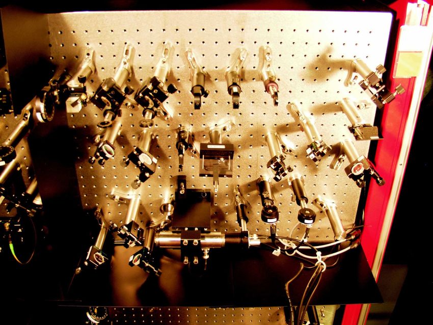
Experimental Setup and Procedure
The experimental setup is shown in Fig. 10. The photograph and the corre-
sponding schematic in Fig.7, show the home-built diode laser in its acrylic-
glass housing. The elliptical light beam emitted from the laser is sent through
an anamorphic prism pair, after which the beam is - to a good approximation
- round in shape. Next, the beam passes through a telescope, which reduces
the beam diameter to fit the aperture of the Faraday isolator. The Faraday
isolator acts as the optical analogue of a normal diode: it prevents the beam
from being reflected back into the laser. Such back reflections can lead to
16photodiodes
Fabry Perot PD1 PD2
Interferometer
neutral
density
filter
beam
stop
l/2 Rb spec. cell
pol. beam cube telescope aperture
Fabry Perot
PD1 PD2
neutral density
neutral density filter
filter
spec. cell
apertures
l/2 & beamcube
beam spliters
Figure 10: Experimental setup.
17unstable behaviour of the laser. For more details on Faraday isolators, see
for example [6]. The laser beam is then divided up by a combination of a
λ/2-waveplate and a polarizing beam cube: the former rotates the (linear)
polarization of the laser beam, whereas the latter’s transmission is polariza-
tion dependent. For more detailed information on the working principles of
polarization optics, see [7]. The position of the waveplate is chosen such that
a small fraction of the laser power goes straight through the beam cube and
into an optical fiber. The fiber is connected to a wavemeter in the lab next
door, such that the laser wavelength can be monitored. The main part of the
laser power is deflected by the beam cube and is available for the Doppler-
free saturation spectroscopy.
The spectrocopy setup is shown in a photograph and a corresponding schematic
in Fig. 10. There are two main beam lines. Again, a combination of a λ/2
waveplate and a polarizing beam cube splits the beam into two. The de-
flected beam goes directly into the Fabry-Perot interferometer and is already
properly aligned. From the beam passing straight through the beam cube,
three beams for saturation spectroscopy are derived. Two weak probe beams
(one for reference purposes which will become clear later) are generated by
inserting two 10 : 90 beam splitters into the ”high-power” (a few mW) pump
beam. At each beam splitter two reflections, one coming from the back and
one from the front facet, are generated. The weaker of the two is blocked
using an aperture. In addition, the pump-beam diameter is controlled us-
ing a telescope and an aperture. The power in the pump and probe beams
can be controlled by inserting neutral density filters. A set of filters covering
about three orders of magnitude in attenuation is available. The three beams
are directed through the rubidium vapour cell at the center of the table by
highly reflecting mirrors (HR @780 nm). Unless told otherwise, you are not
supposed to move or readjust the vapour cell!
In the beginning of the experiment, only the Fabry-Perot cavity (including
the beam line), the vapour cell and the two photodiodes are mounted and
should not be moved. Your task is it to set up the three beams for saturation
spectroscopy. The following practical hints will help you:
• First and most important of all: Be careful with the laser light!
It can cause permanent damage to your and your partner’s
eyes. Always think about what you do in view of this danger!
Wear your laser goggles!
18• Laser light at 780 nm lies in the near-infrared part of the spectrum. In
a darkened room, however, light at 780 nm is visible and easily tracked
with the help of a phosphorescent sensor card. Hence, switch off the
room light! In addition, an infrared beam viewer is available.
• The standard beam height in all of our experiments is 5 inches (12.7
cm). Align the beams in that height (except for the reference probe
beam; it passes the vapour cell above the other two beams).
• Before you start mounting the optics, think about how to best place
all the components. As a reference, use the schematic in Fig. 10.
4.2 Alignment and Measurements
Fig. 11 shows three different absorption spectra that can be obtained with the
suggested setup. For recording spectrum 2, the laser frequency was scanned
and only one probe beam was going through the vapour cell. The other two
beams were blocked. Thus, we get a normal Doppler-broadened absorption
spectrum of a weak laser beam. The two peaks correspond to the transition
(5 S1/2 , F = 2 → 5 P3/2 , F = 1, 2, 3) in 87 Rb and to the transition (5 S1/2 , F =
3 → 5 P3/2 , F = 2, 3, 4) in 85 Rb. When, in addition, the strong pump beam
is passing through the cell, we get spectrum 3. Various Lamb dips, most of
which are not fully resolved, appear. However, with only one probe beam
present, the Doppler character remains. Next, the Doppler background can
be removed by using the second probe beam, which should have no spatial
overlap with the pump beam and basically shows an absorption signal like
spectrum 2. Subtracting the signal generated by the second probe beam
from spectrum 3, we obtain spectrum 4, where all the hyperfine transitions
are individually resolved and no Doppler background is visible.
In order to remove the Doppler character completely and to obtain a flat
baseline, careful alignment of the two probe beams is necessary. It is best to
block the pump beam and align the two probe beams first. The signal from
the two photodiodes PD1 and PD2 are subtracted from each other electron-
ically. This is done on the electronics board ”Adder” mentioned above (see
Fig. 9). The gain for one of the signals can be adjusted with a potentiometer
such that the difference signal is null throughout the whole frequency sweep
of the diode laser. Then, introducing the pump beam crossing only one of
the probe beams, produces saturated absorption lines on a flat background.
191
2
3
4
Figure 11: Oscilloscope screen shot. Yellow (1): Laser HV rampe. Blue (2):
Signal of reference beam. Magenta (3): Photodiode signal of probe beam.
Green (4): difference signal
20Try to record spectra like the ones shown in Fig 11. To this end, try different
combinations of pump and probe beam attenuation levels. Since the transi-
tion strenghts are different for 87 Rb and 85 Rb, best results are obtained when
using different combinations of neutral density filters for the two isotopes.
Then, once you have the ”best” combination of filters, quantitatively measure
the frequency separation between the individual peaks in the spectrum by
calibrating the time axis of the oscilloscope using the Fabry-Perot interferom-
eter. For a given speed of the laser frequency ramp, you can directly read off
the x-axis (time) separation between two different Fabry-Perot transmission
peaks on the oscilloscope. (It is best to store the corresponding oscilloscope
traces.) With the known free spectral range of the Fabry-Perot cavity, this
x-axis separation directly translates into a frequency separation.
5 Analysis
• Using the level schemes in Fig. 6, assign a particular hyperfine tran-
sition to each of the lines in your recorded spectra. Matters are more
complicated in the case of multilevel atoms compared to the two-level
case. Therefore instead of three lines, you will find six spectral lines
for each isotope. The additional three lines are called ”cross-over res-
onances”. For each pair of ”normal” lines at frequencies ν1 and ν2 , a
cross-over resonance occurs at frequency (ν1 + ν2 )/2.
• Find an explanation for these cross-over resonances and understand
why they are so strong.
• From the measured line separations, determine a pair of hyperfine cou-
pling constants (A,B) for each isotope. This can be done by subtracting
Equation (24) from itself.
• Estimate the uncertainty in your results and compare your measured
values for (A,B) to the accepted values in literature (see e.g. Ref. [3]).
References
[1] T. W. Hänsch, A. L. Schawlow, and G. W. Series. The spectrum of atomic
hydrogen. Scientific American, 240:72, 1979.
21[2] W. Demtröder. Laserspektroskopie. Springer, Heidelberg, 1991.
[3] E. Arimondo, M. Inguscio, and P. Violino. Experimental determinations
of the hyperfine structure in the alkali atoms. Rev. Mod. Phys., 49:31,
1977.
[4] P. W. Milonni and J. H. Eberly. Lasers. Wiley-Interscience, New York,
1988.
[5] P. Zorabedian. Tunable external-cavity semiconductor lasers. In F. J.
Duarte, editor, Tunable Lasers, pages 349–442. Academic Press, London,
1995.
[6] L. Bergmann and C. Schäfer. Lehrbuch der Experimentalphysik, Band 3,
Optik. de Gruyter, Berlin, 1993.
[7] W. Demtröder. Experimentalphysik 2. Springer, Berlin, 2002.
A Tools
neutral alignement infrared
density tool sensor
filters card
screw
ball infrared driver
driver viewer
Figure 12: Important tools for setting up the experiment.
22You can also read